1 - Oscillations, sinusoids, and angles#
Waves are fundamental to many areas of physics. For example, they underpin the whole of quantum mechanics and are crucial to our understanding of electromagnetic radiation. Closely related to waves are oscillations, not only because an oscillator can be a source of waves, but also because a wave can be described as a series of interacting oscillators. So, in the first two lectures of the course, we’ll take a detailed look at oscillators before moving onto waves in Lecture 3.
What are Oscillations?#
An oscillator is something that engages in motion that repeats, and this repeating motion is called an oscillation. A simple example is the motion of a mass on the end of a spring held vertically to tension the spring. Given an initial kick downwards, the mass goes down, then it slows down, stops and returns back up again, overshoots, reaches some maximum height, then goes back to where it started. Then it does the same thing again, and again. Don’t think however that oscillators have to bob up and down in front of your eyes. Many physical quantities can oscillate, not just in position, but in other measurable quantities. For example, the mains voltage in wall sockets oscillates even though it can’t be seen at all. Oscillating electric and magnetic fields are the building blocks of the waves that carry light or mobile phone signals. Gravitational waves cause spacetime itself to oscillate. Electrons in atoms oscillate, though these oscillations are not directly observable and have some unusual features that need entirely new physics - quantum physics - to describe. The one recurring theme is that an oscillation is something varying cyclically.
A mass on a spring is an example of a harmonic, or sinusoidal oscillator. In physics we often use mathematics to model behaviour that we measure in experiments. We could do an experiment to record the motion of a mass on a spring. This is an experiment that is easier to think about than to do in practice (Einstein called this kind of experiment a gedanken (thought) experiment). Think of a mass on a spring having a pen attached to it that is drawing on a parchment on rollers as it passes by. The parchment moves from right to left, so that the pen makes a trace as the mass moves up and down. The figure shows what this looks like after a few cycles of the oscillator.
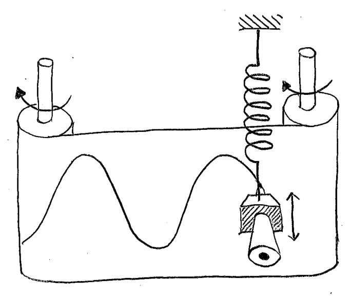
Fig. 1 A gedanken (thought) experiment for plotting the motion of an oscillator on a graph.#
Notice that the trace records the motion of the mass as a function of time. Later motion appears further to the right on the paper; earlier motion is further to the left. The shape of the curve on the parchment is something you have seen before in mathematics, where a similar shape can be obtained by writing something like
The plots of \(y\) as a function of \(x\) corresponding to Equations (1) are shown in Fig. 2.
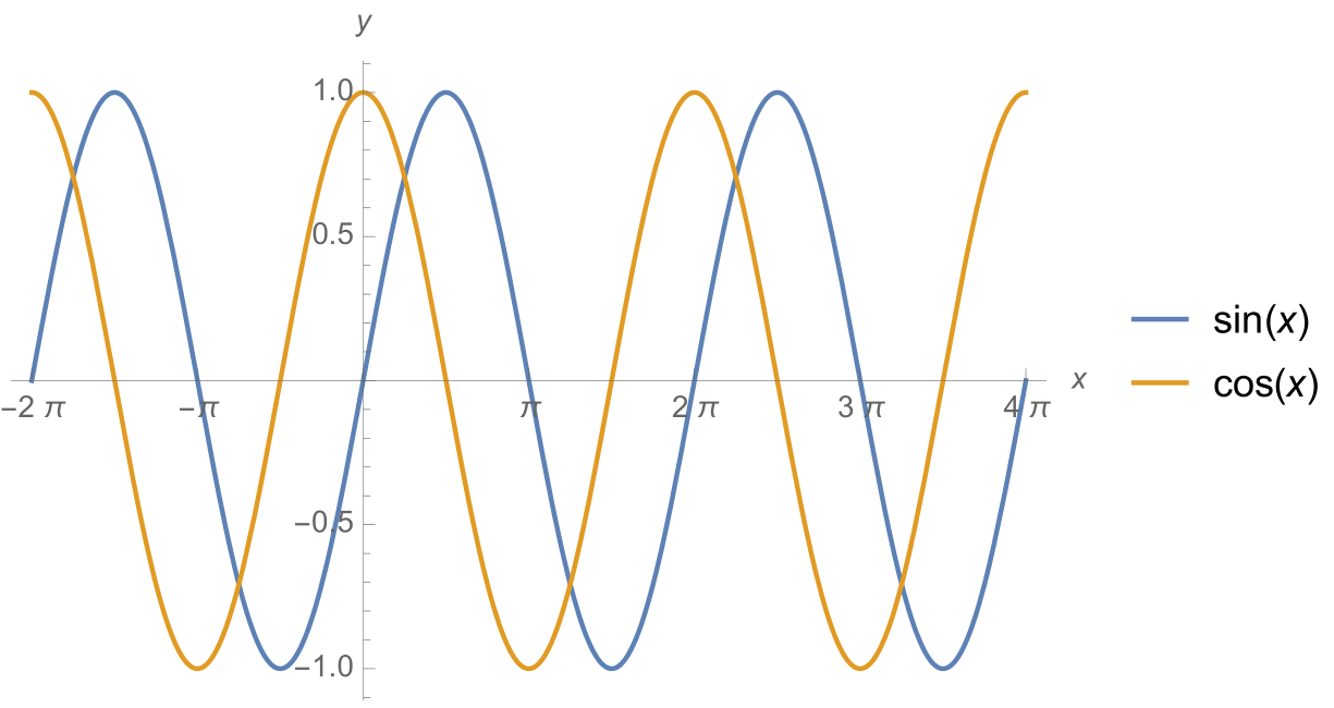
Fig. 2 Plots of \(y=\sin(x)\) and \(y=\cos(x)\).#
These curves both look like the plot showing the motion of our mass-on-spring oscillator. The only difference between them is where the origin is placed. This is why this kind of oscillation is called a sinusoidal oscillation, because the trajectory is well modelled by the functions \(y=\sin(x)\) and \(y=\cos(x)\).
Other words for sinusoidal oscillation are simple harmonic motion, or just harmonic motion, or harmonic oscillations. In this course, all the oscillations we will study are harmonic. Next year you will study other oscillators where the motion is still cyclic, but the motion is not modelled by a single sine wave. Another word for cyclic is periodic.
Relating oscillations to circular motion#
Why does the sine function represent physical oscillators so well? For one answer, recall the original purpose of \(\sin\), which is to relate angles to the ratios of the lengths of sides of triangles. To help visualise this, consider Fig. Fig. 3. Here we have a point that is travelling around some circle at a constant speed – think of a matchstick stuck vertically to a vinyl record player. If you look at the motion of this point side-on, it appears to be making a harmonic oscillation. This works whether you look from the direction of the \(x\)-axis, or the \(y\)-axis, or from any other point in the plane of the circular motion. This leads to a very important feature of harmonic motion:
A sinusoidal oscillation can be thought of as a projection of circular motion in the plane of the circle
You can see that this works geometrically by considering a triangle that has its corners (or vertices) at the origin, the point in question, and the position on the \(x\)-axis directly below the point in question. If the radius of the circle is \(R\), then the equation for the \(x\)-coordinate of this point is \(x=R\cos(\phi)\), where \(\phi\) is the angle between the \(x\)-axis and the hypotenuse of the triangle, and the hypotenuse is of length \(R\). Provided that the angle \(\phi\) increases at a constant rate (i.e., \(\phi(t)=\omega t\), where \(\omega\) is a constant), then the position along the \(x\)-axis will vary according to \(x(t)=R\cos(\omega t)\).
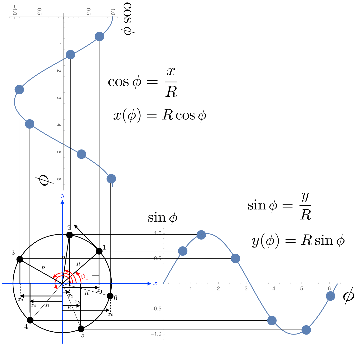
Fig. 3 Trigonometry with triangles constructed inside a circle to different points on the circle, together with the projections of those points horizontally and vertically.#
Key Jargon
Phase: In the case of an oscillator, the value inside the \(\cos\) or \(\sin\) (e.g., \(\phi\) in \(\cos(\phi)\)) is known as the phase of the oscillation.
A note on measuring angles#
In the previous section, we saw how harmonic oscillations are fundamentally related to circular motion, and that the time-dependent position of an oscillator (e.g., \(x(t)\) can be described in terms of angles (e.g., \(\phi(t)\)). As such, angles are crucial to our understanding of harmonic motion, so the system we use to measure angles is of great importance.
You will be familiar with using degrees to measure angles. Degrees is the measures of angle on a protractor, as reproduced in Fig. 4. To measure an angle, you place the crosshairs at the centre of the straight side of the protractor on the point about which the angle will be measured, and around the rim of the protractor the angle measurements are marked off by closely spaced rulings representing degrees. There are \(360^\circ\) in a full circular arc about the cross hairs, or \(90^\circ\) in a right angle. The number of degrees in a full circle is a matter of convention – it is rather arbitrary.
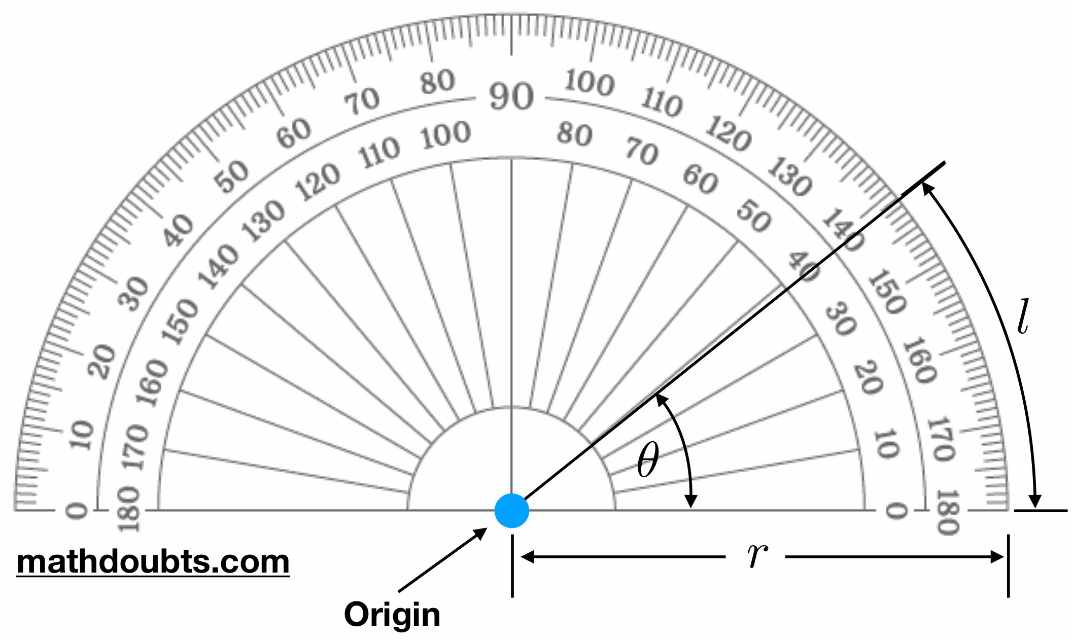
Fig. 4 A \(180^\circ\) protractor for measuring angles in degrees.#
A less arbitrary way of measuring angle is as follows. Take the radius of your protractor as \(r\). One can imagine drawing an arc along the curved part of the protractor whose length is exactly equal to \(r\). Next, draw two straight lines – one from each end of your arc to the protractor’s centre – labelled origin in Fig. 4. The angle subtended by those two lines is exactly one radian.
Now that we’ve defined a radian, we can use it to measure any angle. An angle of half a radian would correspond to when the length of the arc is half that of the radius, while 1.764 radians (to be completely arbitrary) radians would correspond to when the length of the arc is 1.764 times the radius. Of course, if you then take your eraser and rub-out the arc, the angle it still exists, meaning one can use radians to measure any angle, just as one can with degrees.
A full circle corresponds to an arc length that is equal to the circumference of the circle, which is \(2\pi r\). Therefore, the angle in radians that corresponds to \(360^\circ\) is \(2\pi\). Notice that if the protractor gets bigger both the circumference and the radius grow in the same proportion so – just like degrees – angles measured in radians do not depend on the size of the measuring protractor. A \(90^\circ\) right-angle is a quarter of the circumference, which is a distance of \(2\pi r/4=\pi r/2\), meaning that \(90^\circ\) is \(\pi/2\) radians. Similarly, \(180^\circ\) is \(\pi\) radians, and so on. In this course, angles will be in radians unless I explicitly state otherwise.
To convert an angle from degrees to radians, multiply it by \(\pi/180\). Your calculator can calculate \(\sin\) and \(\cos\) of an angle in radians but only if you switch the mode of your calculator to RAD rather than DEG. Try doing this, then check that the cosine of \(\pi/2\) is zero to make sure you have done it right.
There’s one more useful fact about angles in radians that is under-utilised by students: if you are given an angle of \(\theta\) radians and a distance \(l\), then you can very easily work out the length of arc, \(s\), that \(\theta\) corresponds to:
This simple relationship is used over and over again in physics analysis. It is particularly useful when \(\theta\) is a very small angle, when it can be used as a short cut to avoid trigonometry where triangles are very thin slivers. As you’ll see throughout your degree, this trick helps us to make all kinds of approximations that save time and even make otherwise very difficult problems tractable.
Finally, it is also easy to see that when the angle \(\phi\) gets to \(2\pi\) radians, or \(360^\circ\), it can be regarded as going back to zero and starting to rise again, or continuing to increase above \(2\pi\) radians. Therefore, both \(\sin(\phi)\) and \(\cos(\phi)\) are periodic, with period \(2\pi\). In mathematical terms, we write
where \(n\) is any whole number, positive or negative.
Mathematical modelling of oscillations#
So far we have mostly been doing maths. Now we must use the maths we have learned to do physics. We’ve seen how the shapes of the functions \(\sin(\phi)\) and \(\cos(\phi)\) are – for reasons we’ll see in the next lecture – good representations of harmonic oscillations we see in nature. But is that enough? If you type \(\sin(0.32)\) into your calculator you’ll get the answer 0.315… But 0.315… whats? The trigonometric functions return unitless numbers. This is because they represent the ratio of two lengths (e.g., \(\sin(\theta) = {\rm opposite}/{\rm hypotenuse}\)) which is unitless since the length units cancel out.
Amplitude#
In physics, oscillations have a physical meaning; for example, a mass-on-spring moves through a distance measurable in metres, whereas the potential different of an alternating current is measurable in Volts. The size of those oscillations can be big or small, meaning the amplitude of an oscillation is important, and the units of that amplitude must match the units in which the oscillating quantity is measured. For the mass-on-spring, the units of the amplitude could be metres, in which case the ‘dimensions’ of the amplitude are length. Whatever is oscillating, the ‘peak amplitude’ of the oscillation, in units appropriate to what is oscillating, multiplies the \(\sin\) or \(\cos\) function modelling the oscillation. In general, we will use \(\Psi(t)\) to represent the displacement of the oscillator from its equilibrium value at time \(t\), and \(\Psi_0\) will represent the peak amplitude of the oscillator.
Frequency#
Furthermore, oscillations may be rapid or slow. The period of an oscillation is the time taken for one cycle of the oscillation. Somehow, we need to arrange things so that as the time variable \(t\) increases through one period, \(T\), the phase, \(\phi\), of the \(\sin\) or \(\cos\) function increases by \(2\pi\). This requirement is satisfied by writing \(\phi=2\pi t/T\), so that the mathematical model of our oscillation becomes
or perhaps
The sharp-eyed among you will have noticed that there are two symbols representing ‘time’ in Eqns. (4) and (5): \(t\) on the top row and \(T\) on the bottom row. Again, this means that the units (e.g., seconds) cancel each other out, meaning what is inside the \(\sin\) and \(\cos\) brackets is unitless. This is very important: only unitless quantities can go inside the trigonometric functions. ‘But what about radians and degrees - aren’t they units?!’ you cry. Well, look at the mathematical definition of radians expressed in Eq. (2). On the right-hand-side of that equation is a length divided by a length, so the units cancel. So while we may attribute the name ‘radian’ to an angle, it is, in fact, unitless. The same applies to degrees, since degrees is just radians multiplied by a unitless number: \(180/\pi\). [1]
Reminder: Only unitless values can go inside the brackets of the trigonometric functions.
Now, back to oscillations… the frequency of an oscillation is the number of cycles of the oscillation in one second. Frequecy is normally expression in units of Hertz, or Hz, which is the inverse unit of the second (i.e., \(1~{\rm Hz}=1~{\rm s^{-1}}\)). Since the time taken for one cycle is the period \(T\), the frequency \(\nu\) is given by
Substituting this into one of the equations for the oscillation - say Equation (4) we can also write the oscillation model as
Similarly for the other expression using \(\sin\) instead of \(\cos\). Another way of expressing frequency is to use the angular frequency, whose symbol is \(\omega\). The angular frequency is the rate of change in the phase of an oscillator, expressed in units of radians per second. To calculate this, substitute \(t=1\)~s into the expression for the phase, \(2\pi\nu t\), and we learn that the angular frequency is
so that the period of the oscillation can be written
Using the angular frequency, we can write particularly compact expressions for our oscillations
or alternatively
Initial conditions: Sine or cosine?#
Expressions (10) and (11) are different, and represent different functions. The sine function is zero when the phase is zero. By contrast, the cosine function is at its maximum positive when the phase is zero. You would use these two oscillation models to cope with two common classes of initial conditions for the oscillator. To see how this works, consider again the mass on a spring. If the mass is pulled downwards or pushed upwards away from its equilibrium position, then released from rest at this displaced position at time \(t=0\), then its initial displacement will be its peak amplitude in the ensuing oscillations. You would then use \(\Psi=\Psi_0\cos(\omega t)\) to model the motion of the mass, because this model has its maximum displacement at time \(t=0\).
In another class of oscillations, the initial displacement of the mass at time \(t=0\) is zero but at time \(t=0\) it is given some initial velocity. So, at time \(t=0\), it is moving, but its displacement from the equilibrium position is zero. In this case you would use \(\Psi=\Psi_0\sin(\omega t)\) to model its subsequent motion, because the \(\sin\) function has zero displacement at zero phase.
Arbitrary phase offsets#
It may have occurred to you from looking at Fig. 2 that any displacement of either \(\sin\) or \(\cos\) along the horizontal axis yields another perfectly valid oscillation. These displacements are achieved by adding a phase offset or phase shift to the argument of the sine or cosine function. So, for example we can write a more general oscillation with an arbitrary phase at time \(t=0\) like this:
You could also use \(\cos\), but it turns out that a particular choice of \(\phi_0\) applied to \(\sin(\omega t + \phi_0)\) is the same as \(\cos(\omega t)\): when \(\phi_0 = \pi/2\).
Key Jargon
Phase shift/offset: A constant value that’s added to or subtracted from the varying phase of an oscillator is known as a phase shift or a phase offset (they’re interchangeable). In the case of \(\cos(\omega t + \phi_0)\), \(\phi_0\) is the phase shift.
Summary#
At the start of this lecture, we considered what we mean by an oscillation and that in this course we’ll specifically by focussing on harmonic oscillators: those that are well-described by either a sine or cosine.
We then looked at why this may be the case by noticing the similarities between oscillating and circular motion. This led us down the path to describing oscillations in terms of angles, or phase.
At this stage, some of you may feel that the connection between harmonic and circular motion is somewhat arbitrary; in the next lecture, we will broach this by exploring at a deeper level why sinusoids describe the motion of these particular types of oscillator.