9 - Damped Waves

Review of lecture 8

Last time we worked out how to use complex exponentials to solve the differential equation for a lossy oscillator. We discovered that the general solution for the motion \(y(x,t)\) of an oscillator in the case of a weak damping force always in the opposite direction to the oscillator motion, and of magnitude proportional to the magnitude of the velocity of the oscillator, is

(124)\[\begin{align} x(t)&=Ae^{-\frac{\Gamma}{2}t}\left(A\cos\omega_d t + B\sin\omega_d t\right), \label{eq:lossyoscillator} \end{align}\]

where the magnitude of the frictional force is given in terms of the velocity \(v\) of the oscillator as \(F_d=-\eta v\), and the coefficient \(\Gamma\) in the solution is \(\Gamma=\eta/m\), where \(m\) is the oscillator mass. Where \(\omega_d\) is the angular frequency of the oscillator, related to the angular frequency \(\omega_0=\sqrt{k/m}\) of the same oscillator in the case of zero damping by

(125)\[\begin{align} \omega_d=\sqrt{\omega_0^2 - \frac{\Gamma^2}{4}}. \label{eq:omegadamped} \end{align}\]

The damping free angular frequency \(\omega_0\) is related to the spring constant \(k\) and the oscillator mass \(m\) by \(\omega_0^2=k/m\), just as for the simple harmonic oscillator we studied earlier. The constants \(A\) and \(B\) in the solutions can be determined by two initial conditions, giving (for example) the velocity and displacement of the oscillating body at time \(t=0\). We also derived the forms of \(x(t)\) for two other cases, one called critically damped, where \(\Gamma=2\omega_0\), when

(126)\[\begin{align} x(t)=Ae^{-\frac{\Gamma}{2}t}, \label{eq:criticallydamped} \end{align}\]

with \(P\) and \(Q\) constant, and the other called overdamped, when \(\Gamma>2\omega_0\), when

(127)\[\begin{align} x(t)=Ce^{-\left(\frac{\Gamma}{2}+\sqrt{\frac{\Gamma^2}{4}-\omega_0^2}\right)t}+De^{-\left(\frac{\Gamma}{2}-\sqrt{\frac{\Gamma^2}{4}-\omega_0^2}\right)t}, \end{align}\]

where again \(C\) and \(D\) are constants determined using two initial conditions. We remarked also that in general a second order differential equation requires you to follow a procedure equivalent to integrating twice to arrive at a family of possible solutions, and these two indefinite integrals (integrals without limits) result in the two constants

Damping in wave terminations

Hopefully by now you have built a wave generator in the lab and shown that you can use it to create standing waves a certain specific frequencies. Maybe some of you have been able to do this, maybe some of you have done it at A-Level; if you haven’t, or if you’d like to just see some footage of standing waves, you can watch examples on YouTube.[1]

As we have studied, standing waves can be thought of as a superposition of two travelling waves having equal amplitudes moving in opposite directions. Often, however, we are more interested in studying travelling waves. In the past, we’ve done this by considering a wave on an very long string; so long, in fact, that the waves never reach the end and get reflected back. In theory, that’s fine. In practice, however, that’s clearly impractical. To study a travelling wave in practice, we must instead eliminate the reflected wave so we can see the incident travelling wave on its own.

To get rid of the reflected wave, we need to absorb the energy of the incident wave so that it is not reflected back along the string. One way of doing this is to dampen the end of the string by attaching it to a dashpot – a device which introduces a frictional force that is proportional to velocity. To picture this, think of the end of the string being attached to a piston that itself has one end sunk into a viscous substance - such as oil or water (see Fig. 18). Let us solve this system by analysing a travelling wave terminated, at \(x=0\), in such a dashpot. What we’re effectively going to do is work out how viscous the substance in the dashpot needs to be to prevent any waves from being reflected.

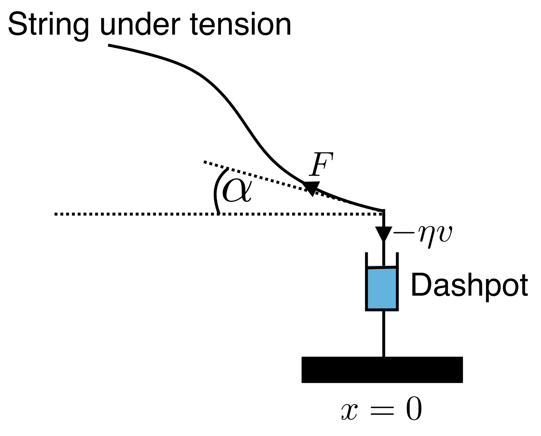
Fig. 18 A wire under tension magnitude \(F\) connected to the end of a piston which causes Stokes’ damping proportional to the velocity of the end of the rope, in a direction opposing the direction of motion.

First, let’s consider the boundary conditions of such a system. The boundary condition is obtained by balancing the forces at the end, i.e., at \(x=0\), of the string in the vertical direction. The two forces acting are the vertical component of the string tension and the damping force opposing the direction of motion. These two forces must balance, since there is no point mass at the end of the string, and a non-zero resultant force on a zero mass would result in an infinite acceleration, which is unphysical. As usual, we write the incident wave propagating down the string to the right, using the complex representation, as

(128)\[\begin{align} \Psi_I(x,t)&=Ae^{i(kx-\omega t)}, \end{align}\]

and the wave reflected off the boundary at \(x=0\) propagating down the string to the left as

(129)\[\begin{align} \Psi_R(x,t)&=Re^{i(-kx-\omega t)}. \end{align}\]

The vertical component of the force on the string is \(F\sin\alpha\) directed upwards. This force must balance the damping force, which when the mass is moving upwards is directed downwards and is of magnitude \(\eta v\), where \(v\) is the magnitude of the velocity of the end of the string and \(\eta\) is the dynamic viscosity, i.e., what we’re trying to calculate. Writing \(\Psi(x,t)\) for the total motion of the string at its end point, we have

(130)\[\begin{align} F\sin\alpha=\eta v. \label{eq:boundary} \end{align}\]

Now, let us as usual analyse the problem assuming the small angle approximation. This means that the angle made by the string with the horizontal is everywhere less than about \(10^\circ\). For these relatively small displacements, we can write

(131)\[\begin{align} \sin\alpha\simeq\tan\alpha\simeq-\frac{\partial \Psi}{\partial x} \end{align}\]

The negative sign on the right is because a negative slope on the string at \(x<0\) results in a positive force upwards. The partial derivative is because \(\Psi\) is a function of both \(x\) and \(t\). Also, the velocity at the end of the string is given by

(132)\[\begin{align} v=\frac{\partial\Psi}{\partial t}. \end{align}\]

Now, there is an additional boundary condition at \(x=0\), which is that the total displacement at \(x=0\) must equal the sum of the contributions from the incident wave \(\Psi_I(x,t)\) and the reflected wave \(\Psi_R(x,t)\). Putting all these things in to Equation (130), we obtain

(133)\[\begin{align} -F\left.\frac{\partial}{\partial x}\left(\Psi_I(x,t)+\Psi_R(x,t)\right)\right|_{x=0}&=\eta\left.\frac{\partial}{\partial t}\left(\Psi_I(x,t)+\Psi_R(x,t)\right)\right|_{x=0} \label{eq:boundary2} \end{align}\]

or

(134)\[\begin{align} -F\left.\frac{\partial}{\partial x}\left(Ae^{i(kx-\omega t)}+Re^{i(-kx-\omega t)}\right)\right|_{x=0}&= \eta\left.\frac{\partial}{\partial t}\left(Ae^{i(kx-\omega t)}+Re^{i(-kx-\omega t)}\right)\right|_{x=0}. \end{align}\]

Doing the derivatives, then setting \(x=0\) and cancelling the common factor of \(e^{i\omega t}\) leads to

(135)\[\begin{align} -F\left(ikA-ikR\right)=-i\omega\eta\left(A+R\right). \end{align}\]

Once again the factors of \(i\) all cancel, so that in this problem there is no parameter-dependent phase shift between the incident and the reflected wave. There could however be a relative minus sign indicating that the incident and reflected signals have opposite phase. The equation becomes

(136)\[\begin{align} -FkA+FkR&=-\eta\omega A-\eta\omega R. \nonumber \\ A(Fk-\eta\omega)&=R(Fk+\eta\omega). \end{align}\]

Rearranging we obtain the following expression for the ratio of the reflected to the incident amplitude.

(137)\[\begin{align} \frac{R}{A}=\frac{Fk-\eta\omega}{Fk+\eta\omega}. \end{align}\]

Let us consider some limiting behaviour of this result to see if it makes sense. You may have found out in the lab that varying the viscosity of the fluid in your wave generator/reflector experiment resulted in different amounts of reflected wave. This result tells us that at a particular value of the reflection coefficient, \(R/A\) goes to zero. This happens when

(138)\[\begin{align} Fk=\eta\omega, \end{align}\]

or

(139)\[\begin{align} \eta=\frac{F}{v} \end{align}\]

Note that the zero reflection point is not at the maximum amount of friction; if we increase \(\eta\) to infinity, corresponding to a really sticky fluid, we obtain \(R/A=-1\), so that all of the incident signal is reflected with the opposite phase. This also happens if you have an infinitely heavy mass on the end of the string, or an infinitely stiff spring. So, there is a particular choice of stickiness of the damping mechanism that leads to perfect attenuation of the reflected wave. Note also that it is not true in general that all the energy in the incoming wave is reflected. This is because the damping mechanism converts some or all of the energy in the incident wave into other forms, such as heat in the viscous medium that makes up the damper.

The physics of this problem is analogous to that of high frequency signals travelling down cables. When you work with oscilloscopes and reasonably high frequency signals, say between \(1\,{\rm MHz}\) and \(1\,{\rm GHz}\), you will have noticed that the cables used are black circular cross section cables, and if you are particularly observant you may have noticed the letters RG-58 written on the outer conductor. This type of cable is coaxial - it consists of an inner conductor that runs down the centre, a dielectric layer that can be made of several different materials, and an outer braided sheath that acts as a ground. This cable is good for carrying sine waves or pulses that have high frequency content, but if the terminations on the end of the cable have the wrong amount of resistance, then some of the incident signal is reflected back down the cable, leading to undesirable standing waves. The way to avoid standing waves is to terminate the cable with an electrical load that matches the characteristics of the cable. RG-58 cable has a so-called ‘characteristic impedance’ of \(50\,{\rm \Omega}\), and it turns out that if you connect a \(50\,{\rm \Omega}\) resistor between the inner conductor and the outer sheath, this results in zero reflection, or a perfect match between the cable and its load. What we have been studying here is the analogous problem in mechanics and waves on strings in particular.

It may occur to you that you might be able to invent a common theory for describing matching between signal transmission lines and loads on the ends of the lines. You will learn about this common theory next year; it is called the theory of impedances.

Summary

In this lecture, we’ve had a quick review of the previous lecture on damped oscillators, then took the next step to look at damped waves. In this latter case, we considered a setup in which a wave was travelling down a wire that was attached to a device that absorbed the energy of the wave. We calculated the conditions under which all the energy of the incident wave was absorbed so that there is no reflected wave. Under these circumstances, no standing wave is set up in the system. We saw that this critical level of damping was dictated by the other properties of the system - notably the tension in the wire and the velocity of the wave. Analogies of this can be drawn with other types of waves, including electrical signals in which you may wish to negate any reflected signals at a terminal.

---

[1]

See, for example, this.