11 - Diffraction and interference

Introduction

In the previous lecture, we looked at the phenomenon of wave interference; specifically the interference of light as it passes through a double slit. By describing the light as waves, and summing the two waves emanating from each slit, we saw that the resulting intensity of the light projected onto a screen is given by:

(155)\[\begin{align} I = I_0\cos^2\left(\frac{\pi d}{\lambda L}y\right) \end{align}\]

where \(I_0\) is the amplitude of the intensity, \(d\) is the distance between the slits, and \(y\) is distance on the screen placed a distance \(L\) from the screen.

One the major assumptions we made in the previous lectures was that the two slits were infinitesimally narrow. While that assumption made the derivation of the intensity profile easier, it’s clearly not practical; how could any light pass through infinitesimally narrow slits? Consequently, in this lecture, we’ll consider the more realistic case of two slits that have a finite width. Before getting to that, however, we’re first going to consider what happens to a wave as it passes through a single finite-width slit.

Diffraction by a single slit

As light – or any other wave – passes through an aperture and hits a screen, it’s natural to think that it simply projects an image of that aperture onto the screen. However, that’s mostly because we’re used to seeing light pass through apertures that are very large in comparison to the wavelength of the light. If, of the other hand, the aperture is comparable to the wavelength of the light, then the waves are instead seen to “spread out” after passing through the aperture in a process called diffraction. In fact, diffraction takes place whenever a wave passes a sharp edge but, in the case of light, this is usually too subtle an effect to witness in everyday life.

To understand why waves get diffracted as they pass through an aperture – or past a sharp edge – we need to look more closely at what actually happens within the aperture itself. Take the case of a slit of finite width. As the wave passes through this slit, it induces oscillations at every point along the slit. Furthermore, all those oscillations are in phase with each other. So, you can think of the slit as containing lots of little oscillators, all oscillating up and down together.

In the case of light – or any other type of wave in two or more dimensions – each one of those little oscillators sends waves outwards radially, as shown in Fig. 22. I like to think of these oscillators as a series of little buoys all in a line on the surface of a calm pond, all bobbing up and down together. Of course, most of those oscillators have neighbouring oscillators either side of them. However, the two at either end – those right at the edge of the aperture – do not. As such, when the waves from those two extreme oscillators spread out radially, they do so beyond the edge of the aperture. It is this radial propagation of waves from each of these “mini-oscillators” within the aperture that causes the “spreading out” effect seen when waves are diffracted as they pass through an aperture.

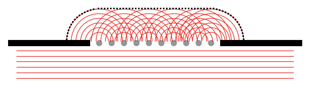
Fig. 22 When a wave passes through single, finite-width slit – in this case from the bottom of the figure upwards – the slit can be thought of as containing an almost infinite number of mini-oscillators (shown here as a limited number of grey circles; in reality, of course, there are almost an infinite number of these mini-oscillators), all moving up an down in phase with one another. Each of these mini-oscillators generates its own set of waves that moves outwards radially (red curves). The net effect of this can be seen as the dotted black line. Directly above the middle of the slit, the net sum of the waves is a plane (straight) wave, but toward the sides the net effect is a curved wave that diffracts around the edge of the slit.

There is, however, another important property of diffraction – one that is very similar to the phenomena of interference that we saw in the last lecture. Since each of those mini-oscillators produces its own set of waves, then those waves interact – or, interfere – with each other. As such, when waves pass through an aperture, not only do they spread out due to diffraction, they also produce an interference pattern. To distinguish this from traditional interference, such patterns are normally called diffraction patterns. And as with interference from a double slit, we can use what we know about waves and borrow some of the concepts from the last lecture to derive an expression the intensity distribution of a diffraction pattern.

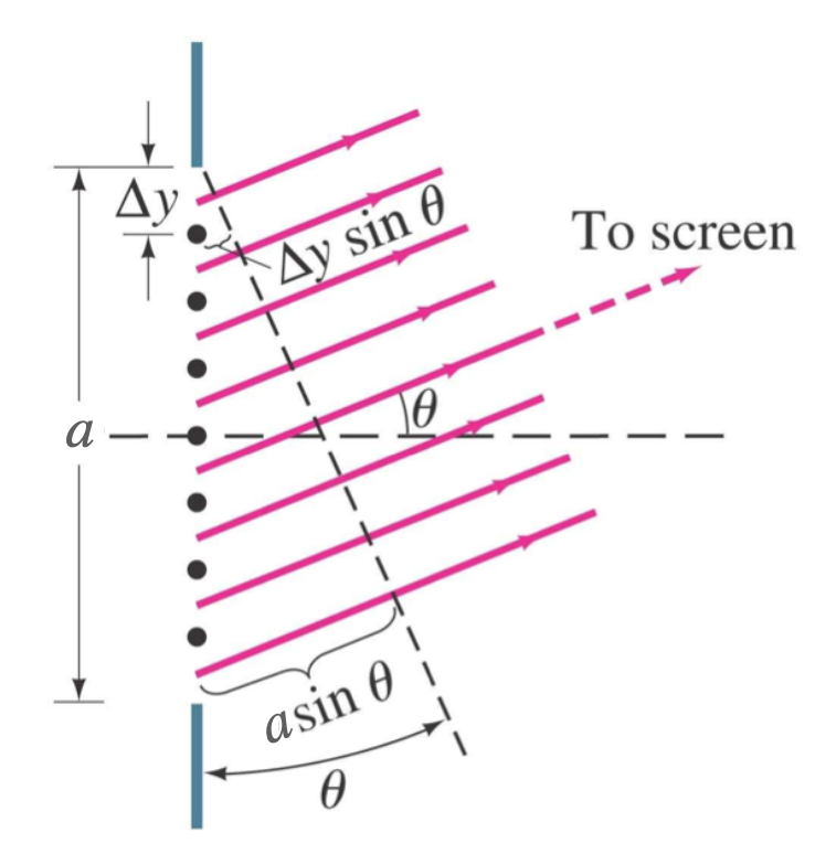
Fig. 23 Diagram showing light waves travelling from left to right through a finite-width slit. As in the previous diagram, the dots show the position of a finite number of mini-oscillators, each separated by a distance, \(\Delta y\). The path difference from the slit to the screen between two neighbouring waves is given by \(\Delta y\sin\theta\), where \(\theta\) is the angle subtended by the light waves to the line normal to the slit.

First, consider the setup shown in Fig. 23, which shows light waves entering a single slit of finite-width, \(a\), from left to right. From there, the diffracted light waves then travel to a screen that is placed a large distance, \(L\), from the slit in comparison to the width of the slit (i.e., \(L>>a\)). As described above, this slit can be thought of as a series of wave-generating mini-oscillators which are transmitting waves radially into the region to the right of the slit. Because they are being transmitted radially, they cover all possible angles but, for the sake of the derivation, let’s just consider a single angle, \(\theta\).[1] If each mini-oscillator is separated by a distance \(\Delta y\) from its neighbour then, by referring to Eq. (146) in the Lecture 10 notes, we can see that the wave from each mini-oscillator – not the oscillator itself – is out of phase from that of its neighbour by an amount:

(156)\[\begin{align} \phi_0 = \frac{2\pi}{\lambda}\Delta y\sin\theta = \beta\Delta y, \end{align}\]

where \(\beta=2\pi\sin(\theta)/\lambda\). As such, if we define \(y=0\) as the middle of the slit, and we also define that the wave from the mini-oscillator at \(y=0\) has a phase shift of zero, then the next few mini-oscillators at \(y=\Delta y, 2\Delta y, 3\Delta y, j\Delta y\) (where \(j\) is an integer) will produce waves with phase shifts of:

(157)\[\begin{align} \phi_1 &= \frac{2\pi}{\lambda}\Delta y\sin\theta = \beta\Delta y\nonumber\\ \phi_2 &= \frac{2\pi}{\lambda}2\Delta y\sin\theta = 2\beta\Delta y\nonumber\\ \phi_3 &= \frac{2\pi}{\lambda}3\Delta y\sin\theta = 3\beta\Delta y\nonumber\\ \phi_j &= \frac{2\pi}{\lambda}j\Delta y\sin\theta = j\beta\Delta y, \end{align}\]

all the way up to:

(158)\[\begin{align} \phi_{N/2} = \frac{2\pi}{\lambda}\frac{N}{2}\Delta y\sin\theta = \frac{N}{2}\beta\Delta y, \end{align}\]

where \(N\) is the total number of mini-oscillators across the whole slit – hence the divide by 2 since we set \(y=0\) as the middle of the slit. Since we’ve only considered half the slit so far, we also need to also consider the waves coming from the middle of the slit downwards. In that case, the \(j\) starts at \(-1\), and progresses through the negative numbers, to \(-N/2\).

To calculate the total displacement at the screen (which, as in Lecture 11, we’ll define as being at \(x=0\)), we need to sum up the displacements from all these waves produced by all these mini-oscillators. Despite having different phase shifts, all have the same angular frequency, wavelength, and amplitude, \(A\), since the whole slit is being illuminated by the same coherent source of light:

(159)\[\begin{align} \psi_{\rm Tot} &= \psi_{-N/2}+\dots+\psi_{-1}+\psi_0+\psi_1+\dots+\psi_{N/2}\nonumber\\ &= Ae^{-i\omega t}(e^{i\phi_{N/2}}+\dots+e^{i\phi_{-1}}+e^{i\phi_0}+e^{i\phi_1}+\dots+e^{i\phi_{N/2}})\nonumber\\ &= Ae^{-i\omega t}\sum_{j=-N/2}^{N/2}e^{i\phi_j}\nonumber\\ &= Ae^{-i\omega t}\sum_{j=-N/2}^{N/2}e^{i \beta j\Delta y}. \end{align}\]

How do we calculate that sum of exponentials? The answer is: we don’t – well, not exactly. Instead, we move away from thinking about the slit as containing lots of discrete oscillators separated from its neighbour by a distance \(\Delta y\), and instead think of it as a continuum, with each infinitesimally small mini-oscillator separated from its neighbour by an infinitesimally small distance, \(dy\). In that case, what is \(N\)? Infinity? Actually, no: it’s important to remember that \(dy\) is infinitesimally small, but not zero. So the number of oscillators is just the width of the slit, \(a\), divided by \(dy\). With that in mind, the sum of the waves from all the oscillators – each separated by a distance \(dy\) – becomes an integral over \(dy\) from the bottom to the top of the slit:

(160)\[\begin{align} \psi_{\rm Tot} &= Ae^{-i\omega t}\int_{-a/2}^{a/2}e^{i\beta y}dy. \label{eq:integral} \end{align}\]

You may ask why \(j\Delta y\) has turned into \(y\) when we move from discrete oscillators to continuous ones? If you think about it, \(j\Delta y\) represents the position of each discrete mini-oscillator along the slit. \(y\) simply does the same job, but in the continuous sense – it just designates the position along the slit.

With the sum now in integral form, it is straightforward to evaluate:

(161)\[\begin{split}\begin{align} \psi_{\rm Tot} &= Ae^{-i\omega t}\int_{-a/2}^{a/2}e^{i\beta y}dy\nonumber\\ &=Ae^{-i\omega t}\frac{1}{i\beta}\left[e^{i\beta y}\right]_{-a/2}^{a/2}\nonumber\\ &=Ae^{-i\omega t}\frac{1}{i\beta}\left(e^{i\beta a/2} - e^{-i\beta a/2}\right)\nonumber\\ &=Ae^{-i\omega t}\frac{1}{i\beta}\left(2i\sin\left(\frac{\beta a}{2}\right)\right)\nonumber\\ &=Ae^{-i\omega t}\frac{\sin(\beta a/2)}{\beta a/2}. \label{eq:sinc} \end{align}\end{split}\]

where in the last step I’ve cancelled the \(i\)’s, and pulled-out a factor of \(1/a\) from the \(A\). I’m allowed to this because both \(A\) and \(a\) are constants for a given system. This form of \(\sin(x)/x\) in Eqn. (161) is also known as \({\rm sinc(x)}\) which evaluates to 1 in the limit of \(x \rightarrow 0\), since \(\sin(x)\) also approaches zero when \(x \rightarrow 0\).

Of course, as with the double slit setup we looked at in Lecture 11, we don’t actually measure the displacement of the wave. Instead, we measure the time-averaged intensity, which is given by:

(162)\[\begin{split}\begin{align} I &\propto \langle\psi_{\rm Tot}^2\rangle\nonumber\\ &= I_0\frac{\sin^2(\beta a/2)}{(\beta a/2)^2}, \label{eq:finsingle} \end{align}\end{split}\]

where the time-average of \((e^{-i\omega t})^2\) is simply \(1/2\) which, together with some other constants, has been absorbed into \(I_0\).[2] This intensity distribution – together with that from an infinitesimally-thin and a finite-width double slit setup – is shown in Fig. 25, toward the end of these notes.

A more realistic double-slit setup

Now that we have encountered the phenomenon of diffraction by a slit of finite width, we can finally tackle the problem of interference by two finite-width slits. Clearly, this is a far more practical setup than the infinitesimally thin slits considered in Lecture 11. As we’ll see, however, it’s no more difficult than applying what we’ve learned from the single-slit example – twice!

Let’s start with a diagram showing two finite-width slits. Fig. 24 shows such a setup. For convenience, we’ll define the point \(y=0\) as being exactly half way between the slits and, as ever, we’ll define \(x=0\) as being the position of the screen. Again, we’ll use \(a\) as the width of each slit (i.e., both slits have the same width), and the centre of the first slit is a distance, \(d\), from the centre of the other. We’ll also assume that \(D>a\). Finally, we’ll define \(L\) as the distance between the slits and the screen and assume \(L>>D\), as we have done so throughout.

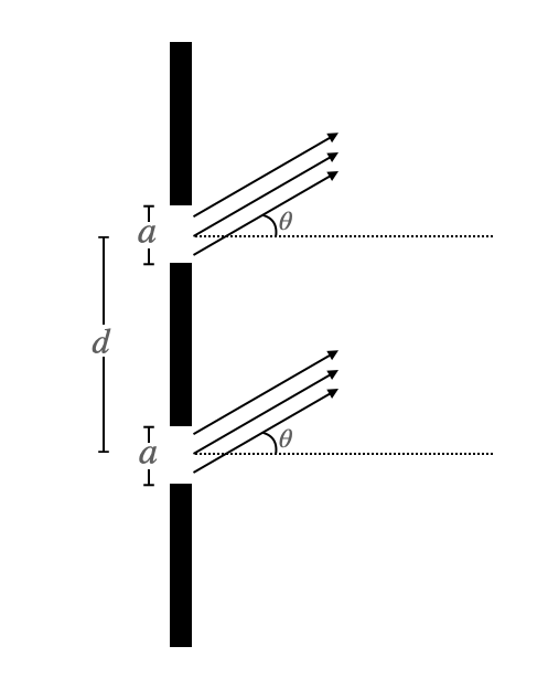
Fig. 24 Diagram showing the double finite-width slit setup. The each slit has a total width of \(a\), and the centre of the top slit is a distance \(d\) from the middle of the bottom slit. Again, I’ve shown the light rays emanating from the slit at an angle \(\theta\) to the line normal to the slits. The screen (not shown) is at a distance, \(L\), which is far to the right of the slits, such that \(L>>d\).

As suggested above, to determine the intensity distribution resulting from light passing through two finite-width slits, we simply need to integrate over all the mini-oscillators within those two openings. Indeed, the only thing that we need to be careful with are the limits of the integration. Based on the geometry of the setup, we can work out that the lower slit extends from \(y=-d-a/2\) to \(y=-d+a/2\) and that the upper slit extends from \(y=d-a/2\) to \(y=d+a/2\). Since no light can be coming from anywhere else, those are the only regions that we need to worry about. So, all we need to do is integrate over each finite-width slit, then add the results together, i.e.,:

(163)\[\begin{align} \phi_{\rm Tot} &= \psi_{\rm Tot1} + \psi_{\rm Tot2}\nonumber\\ &=Ae^{-i\omega t}\left[\int_{-d/2-a/2}^{-d/2+a/2}e^{i\beta y}dy + \int_{d/2-a/2}^{d/2+a/2}e^{i\beta y}dy\right] \end{align}\]

where, again, I’ve assumed that both slits are illuminated by the same, coherent beam of light – hence I can take \(Ae^{-i\omega t}\) out as a common factor.

Performing the above integrals gives:

(164)\[\begin{align} \psi_{\rm Tot} &= Ae^{-i\omega t}\frac{1}{i\beta}\left(\left[e^{i\beta y}\right]_{-d/2-a/2}^{-d/2+a/2} + \left[e^{i\beta y}\right]_{d/2-a/2}^{d/2+a/2}\right)\nonumber\\ &=Ae^{-i\omega t}\frac{1}{i\beta}\left(e^{i\beta (-d/2-a/2)}-e^{i\beta (-d/2+a/2)}+ e^{i\beta (d/2+a/2)}-e^{i\beta(d/2-a/2)}\right)\nonumber\\ &=Ae^{-i\omega t}\frac{1}{i\beta}\left(e^{-i\beta d/2}\left(e^{i\beta a/2}-e^{-i\beta a/2}\right)+e^{i\beta d/2}\left(e^{i\beta a/2}-e^{-i\beta a/2}\right)\right)\nonumber\\ &=Ae^{-i\omega t}\frac{1}{i\beta}\left(e^{i\beta d/2}+e^{-i\beta d/2}\right)\left(e^{i\beta a/2}-e^{-i\beta a/2}\right)\nonumber\\ &=Ae^{-i\omega t}\frac{1}{i\beta}\times2\cos(\beta d/2)\times2i\sin\left(\beta a/2\right)\nonumber\\ &=Ae^{-i\omega t}\cos(\beta d/2)\frac{\sin\left(\beta a/2\right)}{\beta a/2}\nonumber\\ &=Ae^{-i\omega t}\cos(\beta d/2){\rm sinc}(\beta a/2), \end{align}\]

where, again, I’ve manipulated the constant, \(A\), to absorb other constants, and release a factor of \(1/a\).

Again, to obtain an expression for the intensity distribution we need to calculate:

(165)\[\begin{split}\begin{align} I &\propto \langle\psi_{\rm Tot}^2\rangle\nonumber\\ & = I_0\cos^2(\beta d/2){\rm sinc^2}(\beta a/2). \label{eq:findouble} \end{align}\end{split}\]

On comparing Eqn. (165) with Eqn. (162) above and Eqn. (153) from Lecture 10 notes, it should be clear to you that the intensity distribution resulting from light passing through two finite-width slits is equal to the product of the intensity distribution from a single finite-width slit and the intensity distribution from two infinitesimally-thin slits. This is also known as modulation - i.e., the intensity distribution from two finite-width slits is the same as that from two infinitesimally-thin slits modulated by that from a single finite width slit. This modulated intensity distribution is shown in Fig. 25.

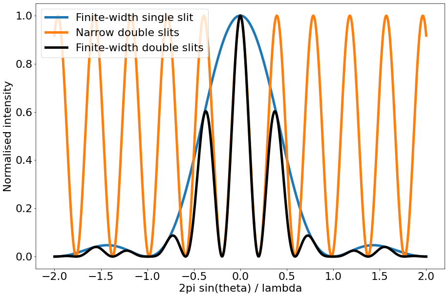
Fig. 25 Plot showing the normalised intensity distribution resulting from the three setups described this and the previous lecture: infinitesimally narrow double slits (orange line), finite-width single slit (blue line), and finite-width double slits (black line). Where applicable, the separation of the two slits is four times the width of the slits (i.e., \(d/a = 4\)). The intensity distribution from the finite-width double slits is that of the narrow double slits modulated by that of the single finite-width slit.

Summary

In this lecture, we’ve expanded our understanding of wave-wave interactions to include diffraction by a single finite-width slit. I think this is a nicer example than the infinitesimally-thin slits encountered in the last lecture, not just because it is more physically meaningful, but because it is also a really good example of how we can use calculus to split up a problem into little pieces then “sum them up” to get the answer. We then went on to use essentially the same approach to determine the intensity distribution resulting from light passing through two finite-width slits.

We have now come to the end of the lecture course – I hope you have enjoyed your first look at oscillations and waves at degree-level. To start with, we looked at oscillators, then expanded this to waves - first in just one dimension, and then in multiple dimensions. Next, we looked at damped oscillators and damped waves, before finally looking at two of the most important features of waves – interference and diffraction – which you will certainly encounter many more times over the next three or four years. But as I’ve said before, just as important as learning about oscillations and waves are the tools that we’ve developed to study them. You’ve learned how to use expansions to approximate, and how that leads to the small-angle approximation, which is one of the most useful approximations in all of physics (I still use it regularly in my own research). You’ve also witnessed the remarkable relation that exists between trigonometry and complex numbers – i.e., Euler’s formula – and, crucially, seen how we can use it to make our lives easier when working out problems related to waves and oscillations.

I’ll now pass you on to Profs. Dan Tovey, Mark Fox, and Pieter Kok who are going to teach you all about Electricity, Magnetism, and Quantum next semester in PHY1002. I’m not due to teach any other first or second year modules, but I look forward to seeing some of your in your third year when you’ll attend the best lecture course in the Universe – Cosmology!

---

[1]

Obviously, \(\theta\) can represent any angle you like, so we are, in effect, doing this for all angles – that’s the the whole concept of algebra!

[2]

See Q&A Session 11 for proof that the time-average of \((e^{-i\omega t})^2\) is \(1/2\).