8 - Lossy oscillators

Review of Euler’s formula

By now, you should have covered Euler’s formula in PHY120. This states that:

(97)\[\begin{align} e^{i\theta} = \cos(\theta) + i\sin(\theta). \label{eq:euler} \end{align}\]

As such, we can represent the motion of an oscillating body as the real part of

(98)\[\begin{align} y(t)=Ae^{i\omega t}, \label{eq:oscbehaviour} \end{align}\]

and the motion of a travelling wave in one dimension can be represented as the real part of

(99)\[\begin{align} \Psi(x,t)=Ae^{i(kx-\omega t)}, \label{eq:wavebehaviour} \end{align}\]

where the wave is travelling in the direction of increasing \(x\). In this lecture, we will see how expressing waves in this way can make it far easier to tackle some problems, and specifically that of a Lossy Oscillator.

Complex analysis of a lossy oscillator

Let us start by first considering the approach we took when we started thinking about waves without loss and consider what our intuition tells us about how lossy oscillators behave. In the case of a lossless oscillator, the motion is an undamped periodic sinusoidal wave, something like \(y(t)=A\cos(\omega t)\) if, for example, the oscillator was released from rest at time \(t=0\).

Now, what will happen if the oscillator is losing a small amount of energy? Perhaps there is air resistance, or energy is lost in the spring or suspension wire through heating as the metal deforms slightly. We might expect that if the oscillator was initially released from rest at an amplitude \(A\), then it would subsequently travel through \(x=0\), reach a maximum negative displacement, then return to positive \(x\) and reach a positive displacement where it was again instantaneously at rest. However, this time the displacement at instantaneous rest might be \(rA\), where \(r\) is a positive number slightly less than 1. Now, at this instant, the configuration of the oscillator is exactly as it was at \(t=0\), only the amplitude at rest is \(rA\) instead of \(A\). The argument can then be repeated, so that the next time the mass comes to rest at positive \(x\), its amplitude will be \(r^2A\), the time after it will be \(r^3A\), and so on. The science is very similar to that with the bouncing ball, only there is one important difference. With the bouncing ball, the time of flight between bounces decreased as the bounces got smaller, because the initial velocity determines the time of flight. With the simple harmonic oscillator without loss, we learned that the period of the oscillator does not depend on the amplitude. So, we might suspect that a damped oscillator would maintain the same frequency even as it lost energy, whereas the bouncing ball bounces with an ever decreasing period as it loses energy each bounce. If the damped oscillator does behave this way, then the amplitude of each oscillation is smaller than the last by the same ratio, but the amplitude never reaches zero, and the period remains the same; hence the oscillations carry on for ever, in theory, whereas the bouncing ball stops bouncing in a finite time, even though it has an infinite number of bounces.

Let us formulate the problem of a lossy oscillator using the laws of mechanics. We consider a body of mass \(m\) on a frictionless table connected to a spring, as shown in Fig. 17. The equilibrium position of the body is at \(x=0\), so that when the body is actually at position \(x\), there is a force \(kx\) directed back towards \(x=0\). There is also a damping force, which we will assume is a so-called Stokes damping, where the damping force is opposite in direction to the motion of the mass, and has magnitude \(\eta v\), where \(v\) is the velocity of the body, and \(\eta\) is the coefficient of Stokes’ friction.

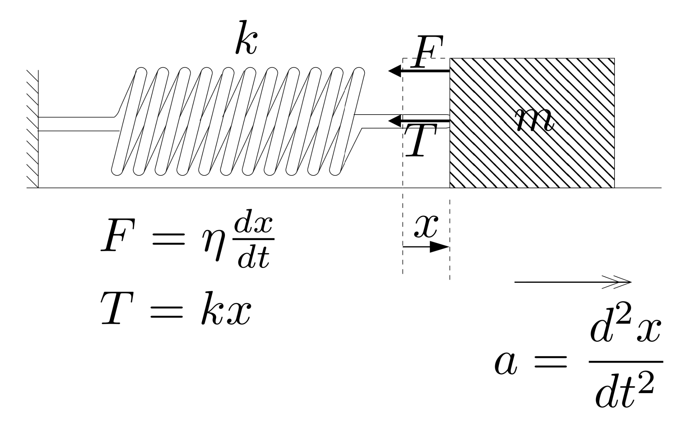
Fig. 17 A damped oscillator with Stokes’ friction - a damping force in the opposite direction to the motion of the body.

Using Newton’s second law, the sum of the forces equals the rate of change of momentum, or \(ma\), where \(a\) is the acceleration of the body. We have

(100)\[\begin{align} ma=-kx-\eta v \label{eq:dampedmotion1} \end{align}\]

Using \(v=\frac{dx}{dt}\) and \(a=\frac{d^2x}{dt^2}\), we get

(101)\[\begin{align} m\frac{d^2x}{dt^2}=-kx-\eta\frac{dx}{dt}. \end{align}\]

Gather all the terms on one side of the equals sign, so that

(102)\[\begin{align} m\frac{d^2x}{dt^2}+\eta\frac{dx}{dt}+kx=0. \end{align}\]

Next, notice that there are constants multiplying all three terms in \(x\). We can get rid of one of these constants by dividing through by it, leading to

(103)\[\begin{align} \frac{d^2x}{dt^2}+\frac{\eta}{m}\frac{dx}{dt}+\frac{k}{m}x=0. \end{align}\]

Finally, we define \(\Gamma=\eta/m\) and \(\omega_0^2=k/m\). The latter definition may seem curious unless you recall that we showed before that in an undamped oscillator made of a mass on a spring, the natural frequency was \(\sqrt{k/m}\), so that this definition of \(\omega_0\) will allow us to compare the frequency of the undamped oscillator with the frequency of the damped one. With these definitions we obtain

(104)\[\begin{align} \frac{d^2x}{dt^2}+\Gamma\frac{dx}{dt}+\omega_0^2x=0. \label{eq:dampedoscillator} \end{align}\]

This is a second order, linear, homogeneous, ordinary differential equation with constant coefficients. What do all these words mean? Second order means that the highest derivative is a second derivative. Linear means that each term contains either the dependent variable (\(x\) here), or a derivative of \(x\) with respect to the independent variable (which is \(t\)); there are no terms containing \(x^2\) or \(x\frac{dx}{dt}\) or \(xt\) or anything complicated like that. Homogeneous means that there is only one dependent variable - which is \(x\) here, and \(x\) depends on \(t\). Constant coefficients means that the coefficients of \(x\), \(dx/dt\) and \(d^2x/dt^2\) are constants (\(\omega_0^2\), \(\Gamma\) and \(1\)); they have no dependence on \(x\) or \(t\).

Solving differential equations is something you will do a lot more of during the course. It turns out that a very large number of physics problems are most easily formulated in terms of differential equations, so that solving them is an important skill. Fortunately, there are actually not so very many differential equations you have to learn how to solve. The damped harmonic oscillator is one of those. You just have to learn about how to solve it and how its solutions behave. So, let’s get stuck in. The easiest way to solve this equation is to assume that the solution takes the form \(x=e^{st}\), where \(s\) is a constant. We use this form because we know that \(e^st\) is an eigenfunction of the operator \(d/dt\), so that every time derivative is going to bring down a factor of \(s\). Let’s substitute in and do it slowly. Let \(x(t)=e^{st}\). Equation (104) becomes

(105)\[\begin{align} \frac{d^2}{dt^2} e^{st} + \Gamma \frac{d}{dt} e^{st} + \omega_0^2 e^{st}=0. \end{align}\]

Since each time derivative brings down a factor of \(s\), because \(e^{st}\) is an eigenfunction of the operator \(d^n/dt^n\) with eigenvalue \(s^n\), we obtain

(106)\[\begin{align} s^2e^{st}+\Gamma s e^{st}+\omega_0^2 e^{st} = 0. \end{align}\]

Dividing through by \(e^{st}\), which is OK because it is never zero for any \(t\), we obtain

(107)\[\begin{align} s^2+\Gamma s + \omega_0^2=0. \label{eq:complimentaryfunction} \end{align}\]

This is an ordinary quadratic equation in \(s\), which we can solve by any of the usual methods. I like to complete the square. To do this write

(108)\[\begin{align} s^2+\Gamma s = \left(s+\frac{\Gamma}{2}\right)^2 - \frac{\Gamma^2}{4}, \end{align}\]

so that Equation (107) becomes

(109)\[\begin{align} \left(s+\frac{\Gamma}{2}\right)^2 + \omega_0^2-\frac{\Gamma^2}{4}=0. \end{align}\]

Taking to the constants to the right of the equals sign, we obtain

(110)\[\begin{align} \left(s+\frac{\Gamma}{2}\right)^2 = -\left(\omega_0^2-\frac{\Gamma^2}{4}\right) \end{align}\]

Note that in the interesting case where the damping is small, the coefficient \(\Gamma\) is very much smaller than \(\omega_0\), so that the right hand side will be negative. However, this should not scare us any more, because we know how to take the square root of a negative number. We obtain

(111)\[\begin{align} s+\frac{\Gamma}{2}=\pm i\sqrt{\omega_0^2-\frac{\Gamma^2}{4}} \end{align}\]

or

(112)\[\begin{align} s=-\frac{\Gamma}{2}\pm i\sqrt{\omega_0^2-\frac{\Gamma^2}{4}}. \end{align}\]

These values of \(s\) are consistent with solutions to Equation (104) of the form \(e^{st}\). Let us see where these solutions lead us. The solutions are

(113)\[\begin{align} x(t)&=e^{-\frac{\Gamma}{2} t \pm i\sqrt{\omega_0^2-\frac{\Gamma^2}{4}}t}. \nonumber \\ &=e^{-\frac{\Gamma}{2}t}e^{\pm i\sqrt{\omega_0^2-\frac{\Gamma^2}{4}}t}. \end{align}\]

Underdamped or slightly damped oscillations

We continue for a while to consider the case where the damping is slight, so that \(\omega_0 \gg \frac{\Gamma^2}{4}\). We can define the variable \(\omega_d = \sqrt{\omega_0^2-\frac{\Gamma^2}{4}}\), which will be positive, and these solutions take the form

(114)\[\begin{align} x(t)=e^{-\frac{\Gamma}{2}t}e^{\pm i\omega_d t}. \label{eq:underdamped1} \end{align}\]

You can see here that the amplitude of the oscillation decays exponentially, because of the real exponential that appears to the left, but that the oscillations themselves continue at a fixed frequency \(\omega_d\), which is slightly less than the frequency of the undamped oscillator \(\omega_0\). However, we are only interested in real solutions. We could just take the real part of this expression, but this would actually only give us one real solution, whereas we know there is a family of real solutions. The whole family is found by taking superpositions of the two solutions for \(s\). The easiest such superposition is to add them with equal coefficients.

(115)\[\begin{align} x_1(t)&=Ae^{-\frac{\Gamma}{2}t}\left(\frac{e^{i\omega_d t}}{2}+\frac{e^{-i\omega_d t}}{2}\right) \nonumber \\ &=Ae^{-\frac{\Gamma}{2}t}\cos(\omega_d t). \end{align}\]

A second real solution is found by subtracting the two possibilities, again with equal coefficients. This solution is a bit more obscure because of the factor of \(i\) that must appear in the denominator by the definition of the \(\sin\) function.

(116)\[\begin{align} x_2(t)&=Be^{-\frac{\Gamma}{2}t}\left(\frac{e^{i\omega_d t}}{2i}-\frac{e^{-i\omega_d t}}{2i}\right) \nonumber \\ &=Be^{-\frac{\Gamma}{2}t}\sin(\omega_d t). \end{align}\]

The most general real solution is a superposition of these two possibilities

(117)\[\begin{align} x(t)=e^{-\frac{\Gamma}{2}t}\left(A\cos(\omega_d t) + B\sin(\omega_d t)\right). \end{align}\]

As for undamped oscillations, the sum of the \(\cos\) and \(\sin\) solutions can also be written as a \(\cos\) solution with a phase shift \(\phi_0\) at time \(t=0\).

(118)\[\begin{align} x(t)=Ae^{-\frac{\Gamma}{2}t}\cos(\omega_d t + \phi_0). \end{align}\]

You can see that these solutions behave as our intuition suggested they might. The frequency of the oscillation, though not quite equal to that of the undamped oscillator, is a constant. You can think of the damping as slowing down the motion of the oscillator, which will increase the period, or decrease the frequency of the oscillation compared to its undamped value. The period of the oscillator is \(T=2\pi/\omega_d\), so that for each period of the oscillator its amplitude will increase to a factor of

(119)\[\begin{align} e^{-\frac{\pi\Gamma}{\omega_d}} \end{align}\]

relative to that in the previous cycle.

Overdamped solutions

There are of course more highly damped possibilities. The first is the overdamped case, where \(\frac{\Gamma^2}{4}>\omega_0^2\). In this case the roots (solutions) of Equation (107) are real, and you get two different real values for \(s\)

(120)\[\begin{align} s=-\frac{\Gamma}{2}\pm\sqrt{\frac{\Gamma^2}{4}-\omega_0^2} \end{align}\]

The motion of the mass is a superposition of these two solutions,

(121)\[\begin{align} x(t)=Ce^{-\left(\frac{\Gamma}{2}+\sqrt{\frac{\Gamma^2}{4}-\omega_0^2}\right)t}+De^{-\left(\frac{\Gamma}{2}-\sqrt{\frac{\Gamma^2}{4}-\omega_0^2}\right)t} \end{align}\]

In this case the damping is so severe that the body fails to oscillate at all. In fact, though it is possible given a very large initial negative velocity that you might force the body to return once to the origin, the subsequent motion of the body after that single return would not bring it back to the origin a second time.

Critically damped solution

One final solution remains to be considered - critical damping. This is the case where \(\frac{\Gamma^2}{4}=\omega_0^2\). In this case the two values of \(s\) solving Equation (107) coincide at

(122)\[\begin{align} s=-\frac{\Gamma}{2}. \end{align}\]

In this case, the general solution takes a special form that still has two unknown constants but only allows for a single value of \(s\) in the exponential. That solution is

(123)\[\begin{align} x(t)=Ae^{-\frac{\Gamma}{2}t}. \end{align}\]

This solution is such that, when released from rest, the body approaches its equilibrium as quickly as physically possible, but without oscillating. This is why the motion is called critically damped. Critical damping is ideal for sensitive instrumentation where the response of the instrument to a signal is to move a mirror or a needle. You don’t want the mechanism to overshoot the final value and oscillate about it for a long time, neither do you want the needle to take forever to to “settle”. You frequently design damping controls on these kinds of apparatus so that you are in the critical damping regime.

Summary

In this lecture, we’ve seen how to solve the equation of motion for a damped oscillator. This is made far easier now that we know that trigonometric functions can be expressed as complex exponentials via Euler’s formula. We first solved the equation of motion in a general sense, then looked at the specific cases of under, over, and critical damping. In each case, the solution made physical sense: in the underdamped case, the damping was insufficient to stop the oscillations, whereas in the overdamped case, the system took a very long time (and in some cases never) to return to equilibrium. When critically damped, a system approaches the equilibrium position as quickly as possible without oscillating.