10 - Interference

Introduction

Earlier in the course, we spent some time looking at what happens when we sum together two waves travelling in opposite directions: left-to-right and right-to-left.[1] The result was a so-called standing wave – one in which all parts of the wave oscillate in phase with each other, and there is no net “movement” left or right. In the last two lectures of the course, we’re going to look at another example wave addition, one in which the waves are moving in (almost) the same direction. When this happens, the waves are referred to as interfering with one another. As such, this type of wave behaviour is known generally as interference.

You likely came across the concept of wave interference during your A-levels. If you did, you may have seen how light waves travelling through two thin slits produced an interference pattern consisting of regions of bright and dark fringes, such as those shown in Fig. 19. Your teacher may have also demonstrated how the bright fringes are produced at angles, \(\theta\), given by:

(140)\[\begin{equation} d\sin\theta = m\lambda \end{equation}\]

where \(m\) is an integer, \(\lambda\) is the wavelength of the wave, and \(d\) is the separation between the two slits.

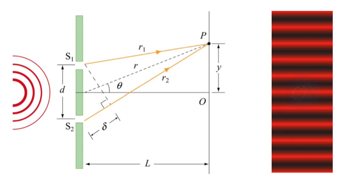
Fig. 19 Left: A double slit experiment. Waves from the left – in this case lightwaves – encounter the double slits, interfere with each other to produce the interference patter shown in the right-hand image.

While deriving the location of the bright fringes is a nice proof, and certainly useful, it’s only part of the story. To get the full picture, we really need to obtain an expression for the full intensity distribution of the interference pattern resulting from light passing through two infinitesimally thin slits. So that is what we’re going to do in this lecture. In the next lecture, we’ll look at the more realistic, but also slightly more difficult, case of interference through a single slit that is not infinitesimally thin. Finally, at the end of the next lecture, we’ll put it all together to consider the interference pattern produced by light waves travelling through two non-infinitesimally thin slits.

Interference by two thin slits

As mentioned in the previous section, our goal is to obtain an expression for the intensity distribution resulting from light waves travelling through two thin slits. To do this, we’ll consider the setup shown in the left-hand diagram of Fig. 19. It should be noted, however, that while we’ll be thinking about this in terms of light waves, all types of wave can undergo interference under the right circumstances, including sound waves, radio waves, water waves etc. As we’ll see later, though, those “circumstances” I refer to are important.

Let us now consider the light waves travelling through the two slits shown in the left hand diagram of Fig. 19. The slits are separated by a distance \(d\), and both slits are located a distance \(L\) from a screen onto which the interference pattern is projected. What should be clear from that diagram is that the distance between the top slit, \(S_1\), and the point \(O\) on the screen is the same as the distance between the bottom slit, \(S_2\), and \(O\). Clearly, this means that waves from both \(S_1\) and \(S_2\) travel the same distance before striking the screen at point \(O\). Now lets consider points upwards of \(O\); specifically, point \(P\). Here, it’s clear that waves from \(S_2\) have to travel further than waves from slit \(S_1\). We can use the cosine law to work out how far each wave travels:

(141)\[\begin{equation} r_1^2 = r^2 + \left(\frac{d}{2}\right)^2 - dr\cos\left(\frac{\pi}{2} -\theta\right) = r^2 + \left(\frac{d}{2}\right)^2 - dr\sin\theta \label{r1} \end{equation}\]

and

(142)\[\begin{equation} r_2^2 = r^2 + \left(\frac{d}{2}\right)^2 - dr\cos\left(\frac{\pi}{2} +\theta\right) = r^2 + \left(\frac{d}{2}\right)^2 + dr\sin\theta. \label{r2} \end{equation}\]

Subtracting Eqn. (141) from Eqn. (142) gives:

(143)\[\begin{equation} r_2^2 - r_1^2 = (r_2 + r_1)(r_2 - r_1) = 2dr\sin\theta \end{equation}\]

and provided that \(L\) is much greater than \(d\) – which it almost always is – then it’s reasonable to say that the sum of \(r_1\) and \(r_2\) is approximately equal to \(2r\), meaning the path difference becomes:

(144)\[\begin{equation} \delta = r_2 - r_1 = d\sin\theta, \label{delta} \end{equation}\]

which can perhaps be more clearly seen by considering Fig. 20 which implicitly assumes \(d<<L\) by displaying \(r_1\) and \(r_2\) as parallel lines.

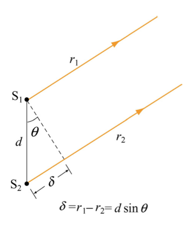
Fig. 20 A zoom-in of a double slit showing the cause of the path difference between two waves emanating from each slit. By showing the path of the waves as parallel lines, this makes the implicit assumption that the separation of the slits are much smaller than the distance between the slits and the screen (the latter of which is not shown here).

The difference in the path lengths between the two slits and point \(P\) is simply a distance. Similarly, the wavelength of a wave is just a distance. As such the difference, \(\delta\), can be written in terms of a number of wavelengths. And this number doesn’t need to be an integer - it could also be a fraction:

(145)\[\begin{equation} \Delta\lambda = \frac{\delta}{\lambda}. \end{equation}\]

Now, thinking back to earlier in the course, one whole wavelength corresponds to a phase difference of \(2\pi\). So, a fractional wavelength corresponds to a phase difference, \(\phi\), of a fraction of \(2\pi\):

(146)\[\begin{equation} \phi = 2\pi\Delta\lambda = 2\pi\frac{\delta}{\lambda} = \frac{2\pi}{\lambda}d\sin\theta. \end{equation}\]

where the last step uses \(\delta = d\sin\theta\) from Eqn. (144).

Now that we have expressed the difference in the path lengths in terms of a phase shift, as opposed to simply a distance, we can write expressions for the waves emanating from each slit:

(147)\[\begin{align} \psi_1(x,t) &= Ae^{i(kx - \omega t)}\\\nonumber \psi_2(x,t,\phi) &= Ae^{i(kx - \omega t + \phi)} \end{align}\]

which, if we conveniently place the screen at \(x=0\), become:

(148)\[\begin{align} \psi_1(t) &= Ae^{-i\omega t}\\\nonumber \psi_2(t,\phi) &= Ae^{i(- \omega t + \phi)}. \end{align}\]

To calculate the total displacement, \(\psi_T(t,\phi)\), at point \(P\) we simply need to sum these two waves, i.e., :

(149)\[\begin{align} \psi_{\rm T}(t, \phi) &= \psi_1(t) + \psi_2(t,\phi)\nonumber\\ &=A(e^{-i\omega t} + e^{i(-\omega t + \phi)})\nonumber\\ &=Ae^{-i\omega t}(1 + e^{i\phi})\nonumber\\ &=Ae^{-i\omega t}e^{i\phi/2}(e^{-i\phi/2}+e^{i\phi/2})\nonumber\\ &=Ae^{i(-\omega t + \phi/2)}(e^{-i\phi/2}+e^{i\phi/2}). \end{align}\]

Now, you may be wondering why I did all that stuff with the \(\phi/2\)’s in the above equations. It was basically so I got a nice trigonometric function out, since \(e^{-i\alpha} + e^{i\alpha}\equiv2\cos\alpha\), i.e., :

(150)\[\begin{align} \psi_{\rm T}(t, \phi) &=Ae^{i(-\omega t + \phi/2})(e^{-i\phi/2}+e^{i\phi/2})\nonumber\\ &=2A\cos\left(\frac{\phi}{2}\right)e^{i(-\omega t + \phi/2)}. \end{align}\]

If I hadn’t done that, I’d have had to mess about with double angle formulas. In the above expression, we’ve got a part that depends entirely on \(\phi\) – the cos part – and a part that depends on both \(t\) and \(\phi\). That last part looks a bit tricky; until, that is, we consider what we actually see when we look at the diffraction pattern. What our eyes (or any other type of detector) actually sees is the time-averaged intensity. Averaged, that is, over a very large number of oscillations. Since intensity is proportional to the square of the displacement, we write the time-averaged intensity as:

(151)\[\begin{split}\begin{align} I &\propto \langle \psi_T^2\rangle\nonumber\\ &\propto4A^2\cos^2\left(\frac{\phi}{2}\right)\langle e^{2i(-\omega t + \phi/2)}\rangle\nonumber\\ &\propto2A^2\cos^2\left(\frac{\phi}{2}\right) \label{intensity} \end{align}\end{split}\]

where the last step comes from the fact that the average value of both \(\cos^2 \alpha\) and \(\sin^2 \alpha\) is 1/2. Clearly, we can replace that proportional sign in Eqn. (151) with a constant of proportionality, \(C\). And since both 2 and A are also constants, we can replace \(2CA\) with a single constant, which we’ll call \(I_0\), meaning:

(152)\[\begin{align} I = I_0 \cos^2\left(\frac{\phi}{2}\right) \end{align}\]

As such, the intensity of light projected onto the screen varies as \(\cos^2\phi\) or, equivalently,

(153)\[\begin{align} I = I_0 \cos^2\left(\frac{\pi d}{\lambda}\sin\theta\right). \end{align}\]

And if \(\theta\) is small (i.e., less than about ten degrees), then \(\sin\theta\approx y/L\), where \(y\) is the distance up the screen, meaning:

(154)\[\begin{align} I = I_0 \cos^2\left(\frac{\pi d}{\lambda L}y\right). \end{align}\]

This intensity profile is shown in Fig. 21.

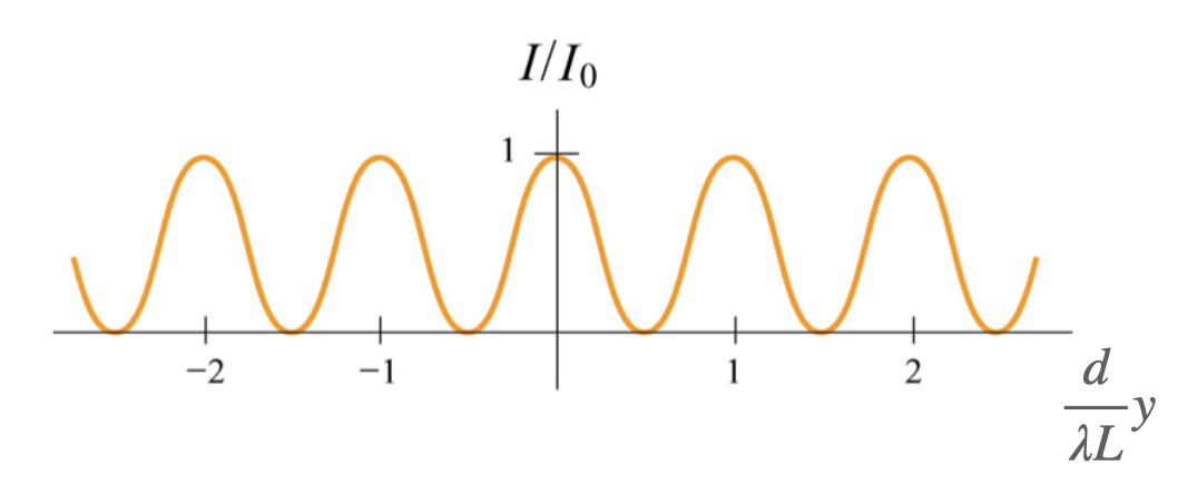
Fig. 21 Plot showing the intensity profile of light passing through two infinitesimally narrow slits of separation, \(d\), projected onto a screen a distance \(L\) away from the slits.

The correct circumstances

We made various assumptions in the above analysis of the intensity profile resulting from lightwaves travelling through a pair of slits. Some of these were mentioned explicitly – such as the requirement that the gaps between the is much smaller than the distance between the slits and the screen – whereas others were more implied. The most important implied assumption is that the waves are coherent, meaning that they are either in-phase with one another, or have a constant phase offset. This is often visualised in terms of the crests of plane parallel waves from the same source hitting both slits at the same time. Or, similarly, the crests of concentric waves from the same source hitting both slits at the same time, as shown in the left-hand diagram of Fig. 19. By contrast, interference patterns are not produced if the waves arriving at each slit are not coherent. All that happens in those circumstances is that light waves consisting of random phase offsets from each slit strike the same point on the screen at the same time. Granted, sometimes they will constructively interfere, but other times they will destructively interfere meaning – and everything in between – so, on average, no overall interference effect is seen.

The other key implied assumption is that both slits are illuminated with lightwaves of the same wavelength, and thus frequency. If this condition isn’t met, then the angular frequencies of the two waves in the above equations will be different; you don’t get interference patterns for effectively the same reasons as why you don’t get interference if the waves are not in-phase.[2] In practice – and prior to the invention of lasers – the coherence requirement is normally achieved by placing a narrow single slit between the light source and the double slits. As light passes through the single slit, it is diffracted so that only coherent waves hit both double slits.

In the next lecture, we’ll look at the case of light passing through a single slit. In doing so, we’ll address another key assumption used in today’s lecture – that of infinitesimally narrow slits which, clearly, are impossible to achieve in practice.

---

[1]

As we have seen, waves don’t have to travel from left to right or right to left, they can travel in any direction they like. I’m just using right-to-left here for ease of description.

[2]

In fact, matching wavelengths is part of the definition of coherent.