3 - Standing waves#
From Oscillators to Waves#
In the previous two lectures we’ve been considering oscillating systems or, more specifically, those that undergo simply harmonic motion. We’ll revisit oscillators later in the course, but for this and the next few lectures we’re going to look at the somewhat related phenomenon of waves. In subsequent lectures, we’ll look at travelling waves – those waves that transport energy from one place to another, whether that’s water waves crossing an ocean, or electromagnetic waves crossing the Universe. To start with, however, we’re going to consider the other main type of wave – standing waves – which, as we’ll see in this lecture, are a sort of half-way-house between an oscillator and travelling wave. This feature makes an an ideal transition between the oscillator and wave sections of the course.
Guitar string standing wave#
The classic example of a standing wave is the guitar string. When one plucks an individual string on a guitar, one sees that the whole string oscillates. However, even if we assume that the guitar string is vibrating harmonically, it is clear that it can not be described mathematically in quite the same way as the harmonic oscillators of the last two lectures. This is because while each small section of the string oscillates harmonically, the amplitude of these mini-oscillators changes along the length of the string. In other words, the amplitude, \(A\), of the oscillations is a function of position, \(x\), meaning that the displacement, \(\psi\), of a tiny section of string at location \(x\) at time \(t\) is given by
where \(\omega\) is the angular frequency of the oscillating string and \(\phi_0\) is a phase shift that I can use to account for the phase of the string at time \(t=0\)\ s. Notice that the displacement, \(\psi(x,t)\), is now a function of both time and position, rather than just time as in the case the oscillators we looked at last week.
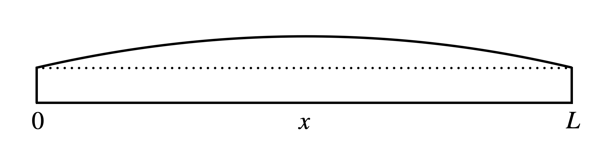
Fig. 6 A vibrating guitar string of length \(L\) captured at its maximum displacement#
With the time-dependence of the string’s motion already defined (i.e., \(\sin(\omega t + \phi_0)\)) we now need to obtain a mathematical expression for \(A(x)\), i.e., how the amplitude of the oscillations of each tiny section of string changes along the whole length of the string. To do this, we’ll consider what the string would look like if we managed to take a high-speed photograph of it while at its maximum vertical displacement, as shown in Fig. 6. Since it is captured at is maximum displacement, this image shows amplitude, \(A(x)\), of the wire at all values of \(x\) from zero to \(L\), where \(L\) is the length of the string. There are three important things to note here about \(A(x)\):
it varies smoothly along the length of the string;
it is zero at position \(x=0\); and
it is zero at position \(x=L\).
The second and third criteria are examples of an extremely important concept in physics – they are what are known as boundary conditions. You will encounter boundary conditions throughout your degree and, as you’ll see, they are really useful for restricting the range of solutions to a problem.
To describe \(A(x)\) in mathematical terms we require a function that satisfies all three of the criteria above. The first criterion is satisfied by any smoothly-varying function, of which there are an infinite number to choose from, so that doesn’t help us much! The second criteria is somewhat more helpful, as it implies that whatever function we choose can’t have an offset at \(x=0\). The third criteria is particularly helpful, however, as it implies that the function must curve back downwards in order to return to zero at \(x=L\). There are a few different functions that satisfy all three criteria[1], but for reasons we’ll encounter later, we will use \(\sin(\theta)\).[2] We do, however, need to be a bit careful about what we put inside the brackets to ensure that it is zero at both \(x=0\) and \(x=L\). Since \(\sin(0)=0\), then provided we don’t have a phase shift inside the brackets, the first boundary condition will be met.
For the second boundary condition, we can turn to the fact that \(\sin(\theta)\) is a repeating function – it returns to zero at \(\theta=\pi\) radians. Therefore, by setting
we ensure that all three criteria are met, since when \(x=L\) only \(\pi\) is left inside the brackets. In Eq. (36) I’ve used \(\psi_0\) to represent the maximum displacement across the entirety of the string, which happens at \(x=L/2\); in other words, \(\psi_0\) is the amplitude of the standing wave.
With \(A(x)\) now defined, we can substitute it into Eq. (35) to obtain the full mathematical expression for the guitar string standing wave shown in Fig. 6:
Multi-modal standing waves#
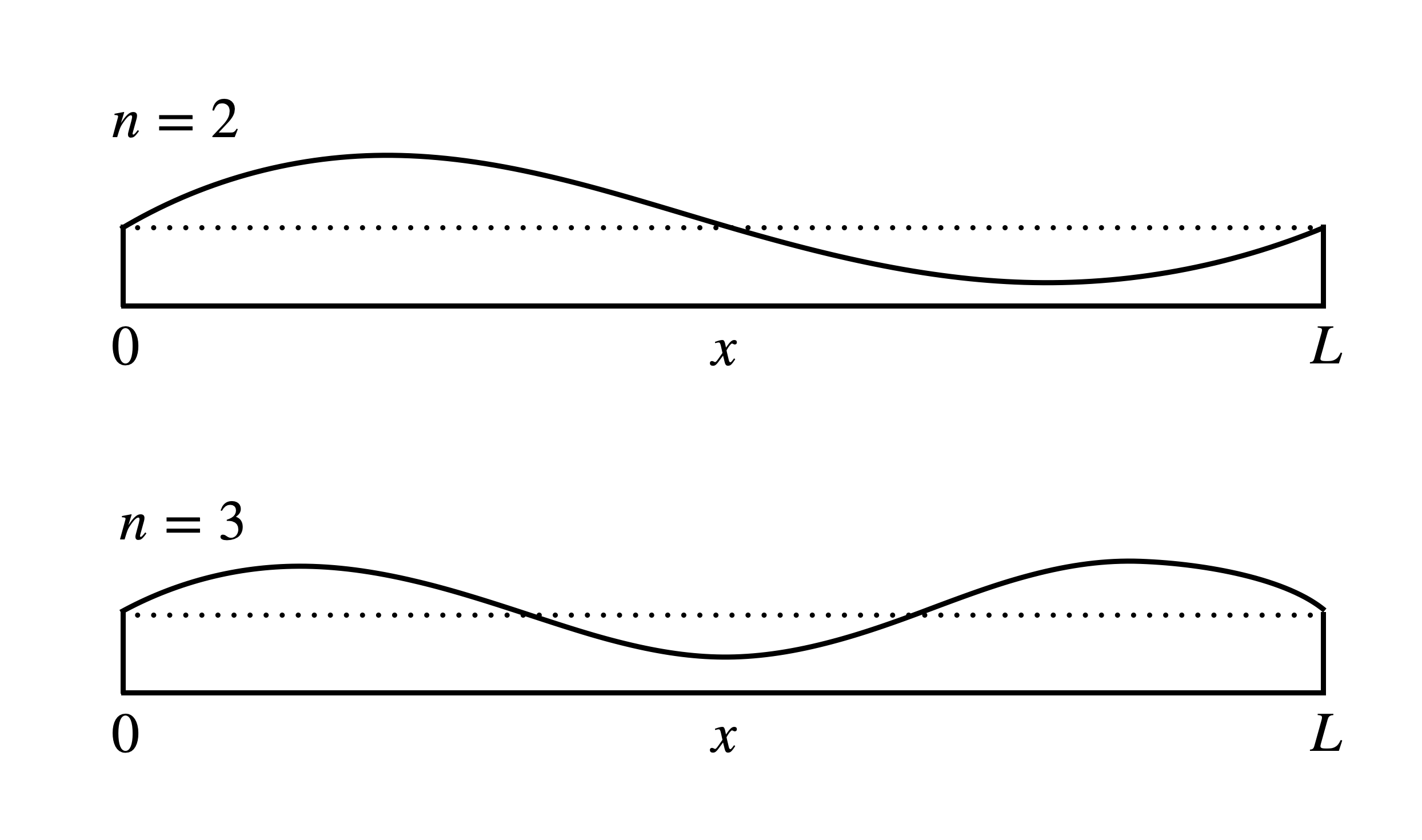
Fig. 7 The second (top) and third (bottom) modes of a vibrating string.#
In the previous section we ensured that the third boundary condition was met by utilising the fact the \(\sin\) function returns to zero when \(\theta=\pi\) radian. However, you’ll be aware that that’s not the only value of \(\theta\) when \(\sin(\theta)=0\). In fact, \(\sin(\theta)=0\) every time \(\theta=n\pi\), where \(n\) is an integer. As such, the following expression for \(A(x)\) also satisfies all three boundary conditions:
where, again, \(n\) can be any integer value. When \(n=1\), we get the first mode of oscillation of the guitar string (as shown in Fig. 6, whereas when \(n=2\) or \(3\) we get the second or third modes shown in Fig. 7, respectively. Looking more closely at the \(n=2\) case, it should be evident that this very much looks like a wave with a wavelength equal to \(L\). From this, it’s easy to see why this phenomena is known as a standing wave – it has the form of a wave, but it doesn’t move any where as it is constrained to the string. In the case of the \(n=3\) example, the standing wave has a wavelength equal to two-thirds \(L\), while the \(n=4\) case would have a wavelength equal to \(L/2\), or \(2L/4\). Continuing this pattern, we can see that the wavelength of each successive mode is given by:
meaning the wavelength is effectively quantised – it can only adopt very specific values dictated by the length, \(L\), of the string. As you’ll see next semester, this forms the basis of all of quantum mechanics!
#Key Jargon
Node: The points on a standing wave where the displacement is always} zero. In the case of the guitar string, the first mode has two nodes, the second has three, the third has four, and so on.
Antinode: The points on a standing wave where the displacement is always maximum. In the case of the guitar string, the first mode has one antinode, the second has two, the third has three, and so on.
If we next rearrange Eq. (39) for \(L\), we get \(L=n\lambda_n/2\), which can substituted into Eq. (38) to obtain:
where I have defined \(k_n = 2\pi/\lambda_n\) which is called the wavenumber of the wave. Of course, this doesn’t alter the fact that the wavelength, \(\lambda_n\), of the standing wave is constrained to certain set values defined by Eq. (39).
Open and closed pipes#
Up to now we’ve only considered one type of standing wave – that which, like a guitar string, has boundary conditions which forces the amplitude of the wave to be zero at both \(x=0\) and \(x=L\). There are, however, two other main types of linear standing waves, those in which the amplitude is:
zero at \(x=0\) and maximum at \(x=L\); and
maximum at both \(x=0\) and \(x=L\).
A physical example of the first is an example of a pipe that is open at one end (at \(x=L\)) but closed at the other. Consider a sound wave being sent down the pipe from the open end toward the closed end. At the point the sound wave hits the closed end, the air molecules are butted-up against the closed end, so they can’t vibrate: their amplitude of vibration is zero. By contrast, an example of the second case is a pipe that is open at both ends.
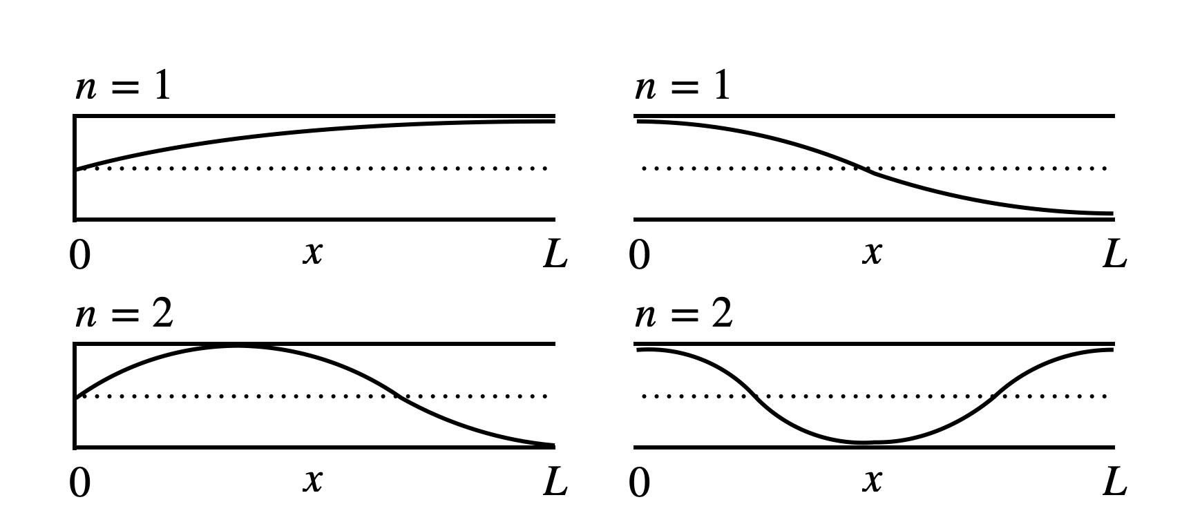
Fig. 8 Left: The first two standing wave modes in a closed-ended pipe. Right: The first two standing wave modes in a open-ended pipe.#
Key Jargon
Wavenumber: The wavenumber of a wave, whether standing or travelling, is defined as \(k=\frac{2\pi}{\lambda}.\) Physically, it tells you about the density of the wave crests. A high wavenumber means the wave crests are bunched-up very closely together.
The diagrams on the left of Fig. 8 shows the first two standing wave modes of a pipe closed at one end. For ease of visualisation I have drawn the sound wave as a transverse wave, rather than a longitudinal wave, but the principle remains the same: there is a node at \(x=0\) and an antinode at \(x=L\). Just as with the guitar string, to ensure that the boundary conditions are always met, the wavelength of the standing wave can only take specific values. In this case, those values are given by:
Just as with the guitar string, since the amplitude of the closed pipe is zero at \(x=0\) then we can again use the \(\sin\) function to model \(x\)-dependent part of the standing wave
By contrast, as right-hand diagrams in Fig. 8 show, we cannot use a \(\sin\) function for the pipe that’s open at both ends, since in this case the amplitude of the wave is a maximum at \(x=0\). Instead, we use a \(\cos\) function which does satisfy this criterion. Again, we need to carefully choose what goes into the \(\cos\) function to make sure it meets the other boundary condition: that it is always at maximum at \(x=L\). This is achieved when
Making sure we use \(\cos\) for the spatially-varying component, this therefore gives the following equation for \(x\)-dependence part of the open-ended pipe standing wave:
The frequency of standing waves#
Up to this point, we’ve largely considered only the \(x\)-dependent part of the standing waves we’ve encountered. However, as Eq. (37) shows, there is also a time-dependent part. Indeed, it should be obvious to anyone who has seen a plucked guitar string that it oscillates in time. Since we started looking at the standing wave modes, I’ve intentionally left-out the time-dependence part of the equations. Now, however, we need to reintroduce the time-dependent parts in order to fully model the standing waves.
As we saw in the last two lectures, we describe the time-dependent part of an oscillator using the frequency, \(\nu\) or angular frequency, \(\omega\), where \(\omega=2\pi\nu\). You should already be aware from A-Levels that the frequency, \(\nu\), and wavelength, \(\lambda\), of a wave are related to one another via the velocity, \(v\), of the wave:
where \(k\) is the wavenumber of the wave.[3] Usually this is thought of in terms of travelling waves, since it’s clear that a travelling wave has a velocity (i.e., it travels within a spatial dimension). However, as we’ll see in Lecture 5, standing waves also have a velocity, and Eq. (45) also holds for standing waves. As such, we can use Eq. (45) to obtain the frequency of a standing wave given its wavelength and velocity.
Since we’ve now obtained expressions for the wavelength of the various types of standing wave, the only part we’re still missing is the velocity. In the case of the sound waves travelling down the open and closed pipes, that velocity part is easy – it is simply the speed of sound in air, \(v_s\), which is constant at a given temperature and pressure. Therefore, the angular frequency of the standing waves in the pipes is given as:
It is important to note that, since \(v_s\) is a constant, Eq. (46) implies that the frequency of the oscillations of a standing wave is also quantised, as well as the wavelength. This feature also applies to the guitar string, since the velocity of a wave in s string or wire is defined by its tension and density. A guitar string of a given density under a given tension can only vibrate at a given set of frequencies, \(\nu_n\). Conversely, this is why the different strings on a guitar produce different notes: even though their length (and therefore first mode wavelength) are all the same, their different densities and tensions cause them to have different sound velocities, meaning they vibrate at different frequencies.
With the fixed set of frequencies now defined, we can finally write down the general equations for the three types of standing wave we have encountered in this lecture:
Closed-closed (e.g., guitar string):
(47)#\[\begin{equation} \psi(x,t) = \psi_0\sin(k_nx)\sin(\omega_nt+\phi_0); \end{equation}\]Closed-open (e.g., pipe closed at \(x=0\), but open at \(x=L\)):
(48)#\[\begin{equation} \psi(x,t) = \psi_0\sin(k_nx)\sin(\omega_nt+\phi_0); {\rm and} \end{equation}\]Open-open (e.g., pipe open at both ends):,
(49)#\[\begin{equation} \psi(x,t) = \psi_0\cos(k_nx)\sin(\omega_nt+\phi_0), \end{equation}\]
where \(k_n=2\pi/\lambda_n\) with \(\lambda_n\) given by Eqs. (39), (41) and (43), and \(\omega_n=2\pi\nu_n\) with \(\nu_n=v/\lambda_n\) (where \(v={\rm velocity}\)).
Summary#
In this lecture we’ve considered standing waves. These are somewhat of a half-way-house between oscillations and travelling waves, the latter we’ll encounter in the next lecture. We saw that standing waves are defined by boundary conditions which constrain their properties. In the case of the guitar string example, these boundary conditions were that the standing wave had to always have zero displacement at \(x=0\) and \(x=L\). By contrast, the open and closed pipes had their own boundary conditions. We also saw how these boundary conditions forced the standing waves to take on a fixed set of wavelengths which, via \(v=\nu\lambda\) implies that they also oscillate at a fixed set of frequencies.