6 - Waves in multiple dimensions

Waves in two dimensions

We are now ready to think about waves propagating in more than one dimension. Such multi-dimensionsal wave propagation is, in fact, far more common in nature than the single-dimension case: think about water waves on the surface of the sea, or sound and light waves propagating in air and space. It is clear that waves propagate in three dimensions, but the maths we have developed so far is not capable of describing them. Fig. 11 shows a picture of some waves travelling towards a beach on a calm day. It is quite a beautiful picture, all those waves peaks and troughs gracefully lined up, all travelling in towards shore, and eventually breaking against the sand. Now, with such a calm day, the waves look almost mathematical, even though they are made of seawater, and probably contain fish, seaweed and crabs.

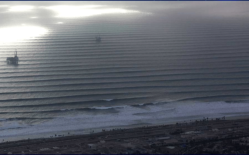
Fig. 11 Waves in an ocean swell. Courtesy: School of Ocean and Earth Science and Technology, University of Hawai’i.

If these are like mathematical waves, what kind of model could we use to describe them? For a start, it is pretty clear that all the points on each wave crest have something in common. Roughly speaking, the displacement of the water surface upwards at each neighbouring point on the wave crest is the same. This means that the phase at each point on the same wave crest is the same as the phase at every other point on the same wave crest. Next, imagine that you are a bird flying above the wave crest. You turn, and fly forwards, catching up with the next wave crest towards the beach. Now, all the points on this crest have the same phase as each other as well. In fact, the phase must differ between two neighbouring wave crests by \(2\pi\), just as it does between two crests of a one dimensional wave on a string. We could also measure the distance between two wave crests, at some moment in time and that would be the wavelength of the wave, \(\lambda\), in which case the wave number would have magnitude \(2\pi/\lambda\), just as it did for our one dimensional waves. This seems reasonably sensible, just treating the two dimensional waves in the same way as we treat one dimensional ones. The only extension necessary is to accept that a line of points, at right angles to the direction in which the wave is moving, has a common phase, since each point on that line has the same displacement due to the wave. This set of points is called a wavefront. In this picture, the wavefronts are straight, and the waves are moving in the same direction everywhere, which is at right angles to the wavefront. These are referred to as two dimensional plane waves. The word plane refers to the fact that the wavefronts are straight. For waves in three dimensions, plane waves have wavefronts that form flat planes; it’s just a generalisation of the two dimensional case we are discussing here.

There are some problems with mathematically modelling such waves. Suppose we view the waves from above - the wavefronts form stripes that are parallel to each other, and those stripes all move in a direction at right angles to the stripes. It is clear that if you freeze time, and move a distance \(\lambda\) in the direction of motion, you will displace yourself forward from one wave crest to the next. However, what happens if you move the same distance in a different direction? If you move a distance \(\lambda\) along the wave front, you will stay on the same wave crest the whole time. There will be no change in the phase of the wave, because all points on the same wave crest have the same phase. What about intermediate directions. Consider Fig. 12.

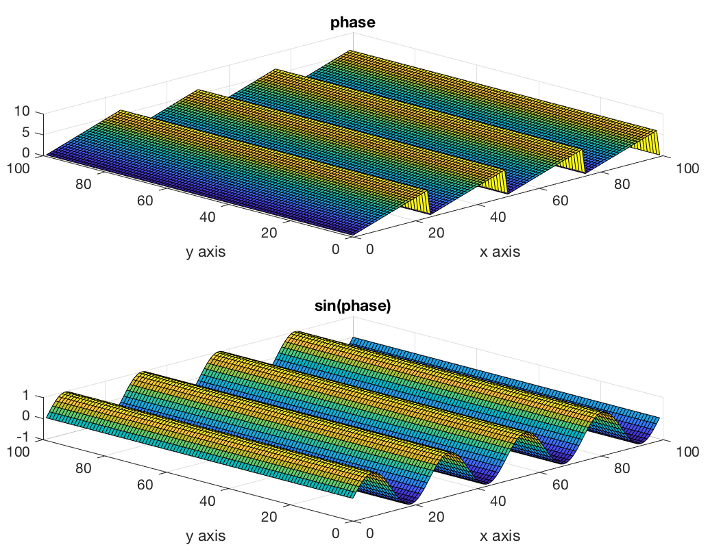
Fig. 12 Wavefronts parallel to the x axis, with constant phase over all values of y at the same x, and the wave displacement shown on the vertical axis. I have also plotted the phase of the wave to show that all points on lines parallel to the wave fronts share a common phase.}

If you displace yourself a distance \(d\) in the \(x\) direction, the phase you move through is \(kd\) radians, where \(k=2\pi/\lambda\), where \(\lambda\) is the wavelength and \(k\) is the wavenumber. It’s exactly the same as the one dimensional case. Now consider, what happens if you move a distance \(d\) in the \(XY\) plane, at an angle \(\theta\) to the \(x\) axis? The component of your displacement resolved parallel to the \(x\) axis is \(d\cos\theta\), hence the phase you have moved through is \(kd\cos\theta\).

Now, we are going to have to model waves which are not parallel to the \(x\) axis, but in other directions. Notice that mathematically \(kd\cos\theta\) is the same thing as \(\vec{k}\cdot\vec{d}\), where \(\vec{k}\) is a vector pointing in the direction of the wave, which is parallel to the \(x\) axis, having magnitude equal to the wavenumber of the wave, and \(\vec{d}\) is the displacement which you are making between the points where you compare the phase. Consider: if \(\vec{d}\) is parallel to the \(y\) axis, then \(\vec{k}\cdot\vec{d}=0\), which is correct because there is no phase change parallel to the wavefront.

The key thing here is the concept of a vector \(\vec{k}\) which is parallel to the direction in which the wave is travelling. Thinking about it, this makes perfect sense - in the case where the wave in one dimension was propagating to the left, we switched the sign of the wavenumber \(k\), which now becomes reversing the direction of the wavevector \(\vec{k}\). To test this, let us invent a different wave vector, say \(k_x = 2\pi(1{\bf i} + 3{\bf j})\). The wavefronts should now be aligned closer to the \(x\) axis than the \(y\) axis, but not perfectly to either of them. This is shown in Fig. 13.

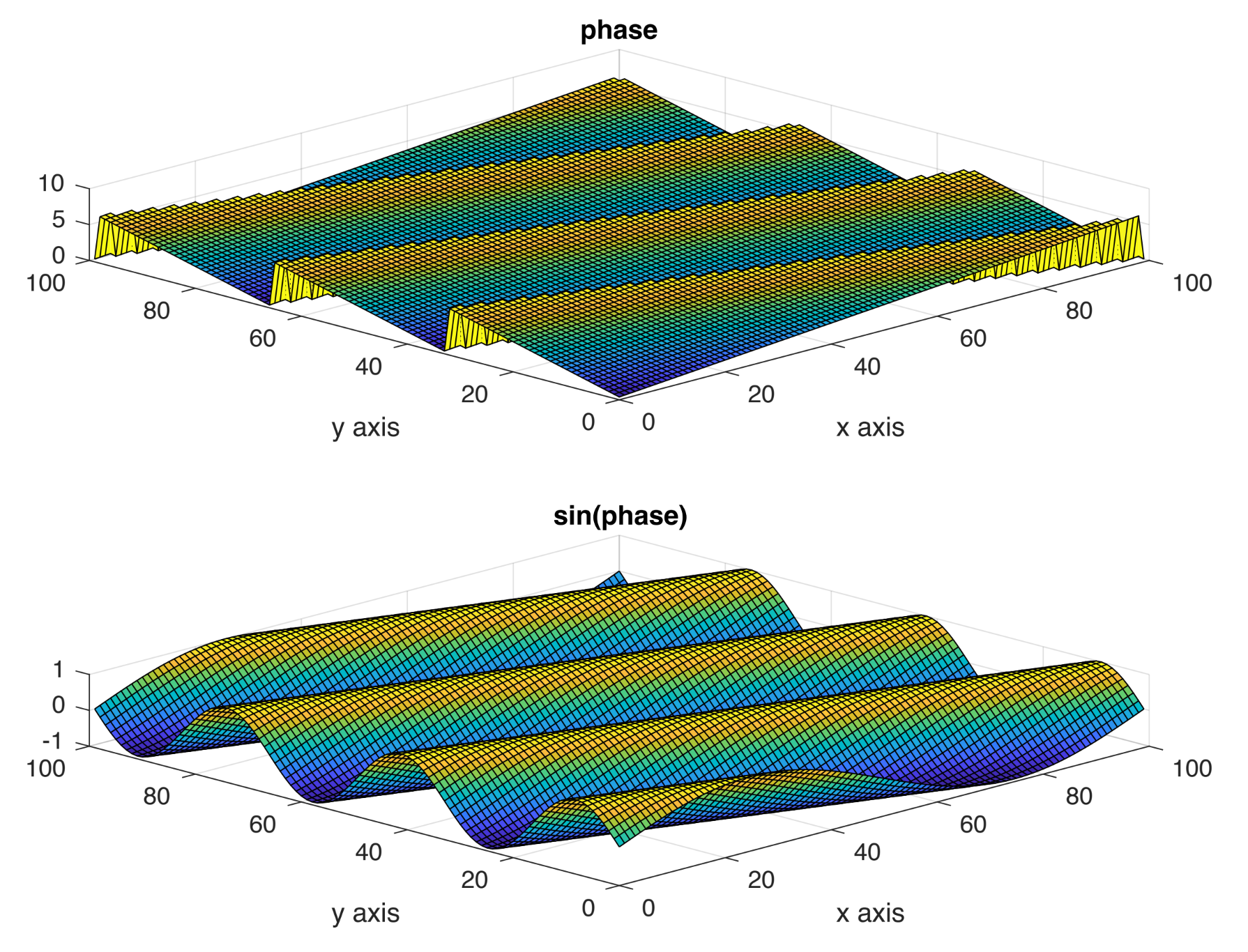
Fig. 13 Waves at wavevector \(k_x = 2\pi(1{\bf i} + 3{\bf j})\).

We therefore arrive at a general way of describing a plane wave moving in an arbitrary direction in the \(XY\) plane. This is

(82)\[\begin{align} \Psi(\vec{x},t)&=\Psi_0\cos(\vec{k}\cdot\vec{r}-\omega t + \phi_0). \label{eq:genwave} \end{align}\]

What are the symbols here? The wavevector \(\vec{k}\) is a vector whose magnitude is the wavenumber of the wave, the number of radians of phase gained per metre of displacement in the direction of the wave, and whose direction is the direction of motion of the wave, which is at right angles to the wave fronts. The vector displacement \(\vec{r}\) is the displacement from the chosen origin of coordinates to the place where the cosine function will calculate the phase of the wave. Note that this vector starts at the origin and goes to any point in space. The dot product ensures that for a plane wave \(\vec{k}\cdot\vec{r}\) will calculate the correct phase shift between the origin and the place in the wave train that \(\vec{r}\) takes you to. The phase offset \(\phi_0\) just allows for the phase of the wave at the origin being something other than zero at time \(t=0\) at the origin.

Geometry of wave vectors

Wave vectors are a curious thing, because they don’t ‘look’ like other vectors that you have seen. Vectors you have met before are visualised directly as arrows in space, quantities with ‘magnitude and direction’ as is often repeated. Forces, for example, are easily represented as arrows, as are velocities, displacements, accelerations, and many of the types of quantities that vectors are used to describe. A wavevector has a somewhat different quality. It is basically a set of parallel lines, or planes in three dimensions, the wavefronts, stacked up one behind the other. The direction of the vector is a line at right angles to these wavefronts, and the magnitude of the vector is the number of these wavefronts per metre, multiplied by \(2\pi\) to convert to radians. Matt will start talking to you soon about potential energy and its relationship to forces. If you’ve ever looked at a topographical map of a mountainous area, you will have seen parallel contours. Each of these contours represents a line of points at a constant height above sea level. If you want to move up the hill as steeply as possible you need to move in a direction at right angles to the contours. The number of contours per unit length in the direction at right angles to the contours is the gradient, or slope, of the hill. So just as wavefronts represent lines of constant phase in a wave train, grid lines are lines of constant height on a map. The gradient of the hill is the rate of change of height with horizontal displacement in the direction of steepest ascent of the hill; the wavenumber of the wave is the rate of change of phase with respect to horizontal displacement in the direction of steepest ascent in the phase.

Constructing a wavevector

There are two key things you need to remember when you construct a wavevector:

• Firstly, its direction is always parallel to the velocity of the wave which, in the case of waves in 2D or 3D, is always perpendicular to the wave front;

• Secondly, the magnitude of the wavevector must always be equal to the wavenumber of the wave.

So, to take a specific example, let’s assume we have a wave of wavelength \(\lambda=0.5~{\rm m}\) travelling across a 2D surface - such as a water wave - with velocity vector \({\bf v}=3\hat{\bf i}+4\hat{\bf j}~{\rm m\, s^{-1}}\). The magnitude of the wave’s velocity. i.e., it’s speed, is \(|{\bf v}|=\sqrt{3^2+4^2}=5~{\rm m\, s^{-1}}\). But what is the wavevector of this wave? As our first rule states, the direction of the wavevector is the same as the velocity vector. The slightly more tricky part is that second rule - we have to make sure that the magnitude of the wavevector is the same as the wavenumber of the wave, i.e., \(|k|=2\pi/\lambda=4\pi~{\rm m^{-1}}\). How do we ensure that? The easiest way is to simply multiply the wavenumber by the unit vector that points in the same direction as the velocity. And since the unit vector is just the vector divided by its magnitude, we get:

(83)\[\begin{align} {\bf k} &= |{\bf k}|\times\frac{1}{\sqrt{3^2+4^2}}(3\hat{\bf i}+4\hat{\bf j})~{\rm m^{-1}}\nonumber \\ &=\frac{2\pi}{\lambda}\frac15(3\hat{\bf i}+4\hat{\bf j})~{\rm m^{-1}}\nonumber \\ &=\frac{4\pi}{5}(3\hat{\bf i}+4\hat{\bf j})~{\rm m^{-1}} \end{align}\]

Please make note of the units in the above equation. Even though we’ve referred to the velocity vector to construct the wavevector, all we’ve really done is taken the direction of the velocity vector (i.e., its unit vector). The dimension of a wavevector is always inverse length (e.g., \({\rm m^{-1}, cm^{-1}}\) etc.)

The case of a wave travelling in three dimensions is the same - you simply multiply the wavenumber by the three-dimensional unit vector, i.e.,

(84)\[\begin{align} {\bf k} = \frac{2\pi}{\lambda}\frac{1}{\sqrt{x^2 + y^2 + z^2}}(x\hat{\bf i}+y\hat{\bf j}+z\hat{\bf k}) \end{align}\]

where \(x,y,z\) describe the direction of the wavevector.

Occasionally, you may need to construct a wavevector using angles instead of a unit vector. For example, a wave may be travelling in a direction that is at an angle \(\theta\) from the x-axis. In that case, you can simply use trigonometry to construct the unit vector, i.e.,

(85)\[\begin{align} {\bf k} &= \frac{2\pi}{\lambda}(\cos(\theta)\hat{\bf i}+\sin(\theta)\hat{\bf j})\nonumber \\ &=\frac{2\pi}{\lambda}\begin{pmatrix} \cos(\theta)\\ \sin(\theta) \end{pmatrix}, \end{align}\]

where I’ve used column vector notation in the second line above. The nice thing about using angles is that you don’t have to divide through by the magnitude to get the unit vector; \((\cos(\theta)\hat{\bf i}+\sin(\theta)\hat{\bf j})\) is already a unit vector.[1]

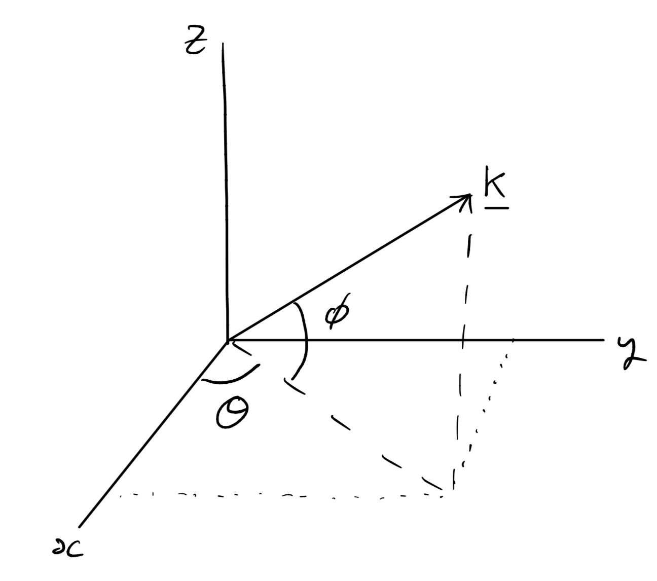
Fig. 14 A vector (in this case a wavevector) directed along a line angled \(\theta\) from the \(x\)-axis and \(\phi\) from the \(x-y\) plane.

Things get slightly trickier if you need to work with angles in three dimensions. Say, for example, that you need to construct a wavevector that is travelling at an angle \(\theta\) from the \(x\) axis, but also \(\phi\) from the \(x-y\) plane. Such a vector is shown in Fig. 14. By referring to that figure, we can see that the \(z\)-component of this vector is simply \(|k|\sin(\phi)\).[2] However, to work out the components in the \(x\) and \(y\) directions, we need to first project the vector onto the \(x-y\) plane. Again, by referring to Fig. 14 we can see that the projection of \({\bf k}\) onto the \(x-y\) plane is \(|k|\cos(\phi)\). To work out the \(x\) component, we need to take that projection and extract its \(x\) component: \(|k|\cos(\phi)\cos(\theta)\). For the \(y\) component, it is \(|k|\cos(\phi)\sin(\theta)\). Therefore, the wavevector of a wave of wavelength \(\lambda\) that is travelling at an angle \(\theta\) from the \(x\) axis, but also \(\phi\) from the \(x-y\) plane is:

(86)\[\begin{align} {\bf k} &= |k|\begin{pmatrix} \cos(\phi)\cos(\theta)\\ \cos(\phi)\sin(\theta)\\ \sin(\phi) \end{pmatrix} \nonumber\\ &=\frac{2\pi}{\lambda}\begin{pmatrix} \cos(\phi)\cos(\theta)\\ \cos(\phi)\sin(\theta)\\ \sin(\phi) \end{pmatrix}, \end{align}\]

where I’ve used column vector notation for compactness.

More arbitrary waves

Of course real waves are not often perfectly parallel straight wavefronts all exactly equally separated. Fig. 15 shows wavefronts in the wake of a boat. I have superposed a sketch of a wavefront, and some wavevectors perpendicular to the wavefronts. Note that \(\vec{k}\) is not in the same direction, and indeed does not have exactly the same magnitude, everywhere on the wavefront. In fact \(\vec{k}\) is a function of position, \(\vec{k}(\vec{r})\). Because \(\vec{k}\) is a function of position, in a complicated wave field like this you would have to do a line integral along a path to figure out the phase shift between two different points,

(87)\[\begin{align} \Delta\phi&=\int \vec{k}\cdot d\vec{r}. \label{eq:funnywavetrain} \end{align}\]

You may not have encountered a line integral before. You’ll certainly see them again during your degree, so I won’t go in too much detail here. All this means, however, is that the total difference in phase between one position and another separated by the displacement \(\vec{R}\) is the sum of all the tiny differences between \(\vec{r}\) and \(\vec{r}+d\vec{r}\) along the entire path.

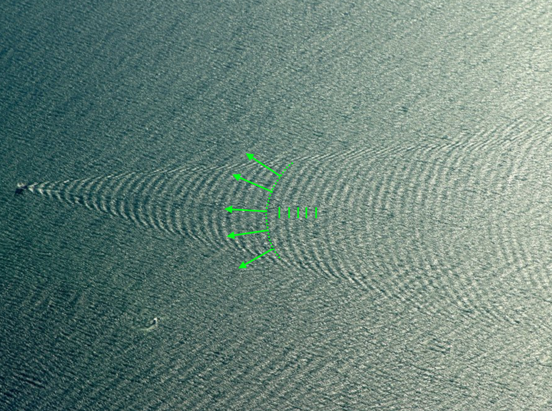
Fig. 15 A boat on the ocean with wavefronts in its wake.

Summary

In this lecture, we’ve moved from considering waves travelling in one dimension (e.g., a transverse wave along a string, or a sound wave travelling in a narrow pipe) to waves travelling in multiple dimensions. For ease of explanation – and figures – we have considered waves travelling on a plane (i.e., two dimensions), with the displacement in the third dimension. However, I’ve intentionally kept the maths rather general, so it should be easy to see how what we’ve covered can also be applied to waves travelling in three dimensions. An example would be a sound waves travelling from a speaker into a room – the wavefronts would form a spherical shell in three dimensions. For a good, if devastating, example of such a three-dimensional wave front, you could watch some of the videos of the explosion that took place at the Port of Beirut in 2020.[3] An explosion is a form of pressure wave, and so similar to a sound wave.

---

[1]

You should be able to show that \((\cos(\theta)\hat{\bf i}+\sin(\theta)\hat{\bf j})\) is a unit vector yourself.

[2]

It may help if you write these components onto Fig. 14 yourself.

[3]

Please note: some people may find such footage distressing.