4 - Travelling Waves

A quick recap

In previous lectures, we’ve looked at the mathematical modelling of oscillations in physics. We ended up with a general formula for an oscillation at frequency \(\nu\) Hz (cycles per second), or angular frequency \(\omega=2\pi\nu\) radians per second, describing how something that is oscillating behaves as a function of time. That general formula can be written in different ways:

(50)\[\begin{split}\begin{align} \psi(t)&=\psi_0\cos(\omega t + \phi_0) \nonumber \\ \psi(t)&=\psi_0\sin(\omega t + \phi_1) \nonumber \\ \label{eq:oscillators} \end{align}\end{split}\]

where \(\phi_0\) and \(\phi_1\) are constant phase shifts.

We also learned in Lecture 1 that when the angle \(\theta\) is in radians, \(\sin\theta = \cos(\theta-\pi/2)\), so that we can relate \(\phi_0\) to \(\phi_1\). Remember that we have moved away from writing \(y(t)\) for the wave amplitude. This is because there are many physical quantities that oscillate. Most of them are not displacements in space, and even those that are can be in any direction, not just up, and in any case, \(y\) doesn’t have to point ‘upwards’. So, we need to get away from the preconception that oscillations can only occur as displacements of objects in space, hence the rather arbitrary symbol \(\psi(t)\) for the oscillating quantity, whatever it is.

Finally, in the previous lecture, we added an extra dimension (literally!) to our considerations by looking at standing waves: oscillators whose displacement depends on both time and position:

(51)\[\begin{align} \psi(x,t) = \psi_0\sin(k_nx)\sin(\omega_nt+\phi_0) \nonumber \\ \psi(x,t) = \psi_0\cos(k_nx)\sin(\omega_nt+\phi_0) \nonumber \\ \end{align}\]

where \(k_n=2\pi/\lambda_n\) is called the wavenumber of the wave and is effectively the number of wavelengths per metre expressed in radians.[1] In this lecture, we will go beyond just thinking about stationary (i.e., standing) waves, to consider the more general case of travelling waves.

Travelling waves

You will remember the picture from Lecture 1 of a roll of paper passing by a mass oscillating up and down on a spring, and how the curve on the paper traces out the sinusoidal motion of the oscillator. Imagining this happening dynamically in front of your eyes, the sine wave passing from right to left is actually in motion in the horizontal direction as the mass bobs up and down. Now, we know of many examples in nature of sinusoidal disturbances in motion. Waves on strings, for example, or waves on the surface of a still pond or canal. We can imagine that the same \(\sin\) and \(\cos\) functions that we use to represent oscillators could also be used to represent these waves in motion. By the end of this lecture, you will know how to do this. But, first, let us try and work out what a moving wave actually is. For a start, the physics underlying waves can be quite different depending on the type of wave motion we are discussing. The actual motion of the water in a wave on a pond or canal, for example, is rather complex.

To understand what a wave is, we consider a specific example of a set of masses connected together by springs. We have neglected gravity, so we assume that there is no gravitational acceleration downwards, but I will still use the words up and down, and I hope you won’t get confused by this. The whole arrangement could also be on a table with no friction, and we are looking downwards on it from above.

In Fig. 9 I have sketched the configuration of masses in in equilibrium. The left hand mass is connected to a drive that can make it go up and down, and the other masses stretch off infinitely to the right of the driven mass.

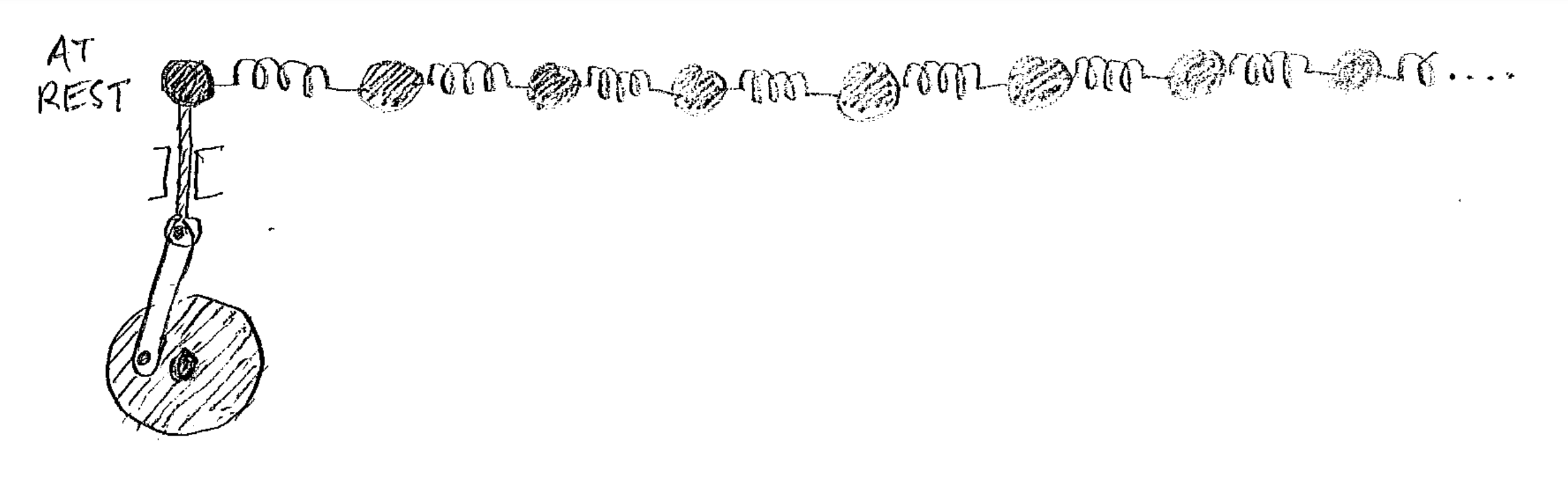
Fig. 9 Some masses connected to their nearest neighbours by springs. One end of the chain is connected to a driver that can cause its mass to oscillate up and down. The rest of the masses stretch off to infinity in a chain to the right of the driven mass. In this picture, the driver is off, and all masses are in their equilibrium positions.

In Fig. 10, the drive has been turned on. As the motor turns, it causes the crank to drive the leftmost mass up and down, so that it is making simple harmonic oscillations. This motion causes waves to travel down the chain of masses from the left to the right, with an amplitude equal to the amplitude of the motion of the driven mass. You can achieve approximately the same effect by waving the end of a long rope up and down with your hand.

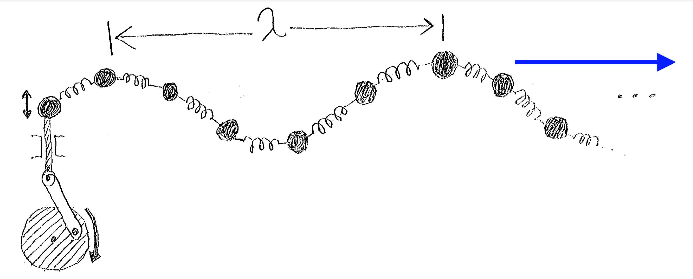
Fig. 10 Once the drive is turned on, the motion of the end mass causes travelling waves to move down the chain of masses from the left to the right. The travelling waves resulting from this have the same character as the trace drawn on the chart recorder by the oscillation recorder discussed in Lecture 1. Here the travelling sinusoidal wave moves in the direction of the blue arrow, to the right.

Now, although the overall motion of the travelling wave is to the right, the individual masses move neither to the right or the left very much, particularly if the amplitude of the wave is much smaller than the wavelength. If you are wondering why this ‘small amplitude’ assumption is necessary, we will return to this later in this course and also in the maths lectures. So, each individual mass moves up and down, but since the masses are connected to each other, the motion of one mass effects that of its neighbours, and hence all the masses oscillate up and down at the same frequency, all move harmonically, but the phase of their motions is connected. This is an example of a type of physical phenomenon called a collective excitation. Collective excitations are very important in many areas of physics. For example, sound waves travel through crystals by exactly this mechanism, where neighbouring ions in a crystal exert forces on each other and these forces can be modelled as springs. Again, more about that later. For now, let’s go on to discuss how to describe a travelling wave mathematically.

A wave at an instant in time

Suppose we take a photograph of the chain of masses at some instant. When we look at the photo, the masses are in the shape of a sine wave in space. Successive photos show that as time evolves, the peaks and troughs of this wave move to the right, but concentrating on just one photo for a minute, you can with your eye measure the distance between successive peaks. This distance is called the wavelength of the wave and it is usually given the symbol \(\lambda\). We have discussed how oscillations are cyclic, with the time between repeats of the cycle called the period of the oscillation and given the symbol \(T\). Now we have waves which, when frozen in time, are periodic in space, with the spatial translation between neighbouring cycles called the wavelength of the wave and given the symbol \(\lambda\). Consider for a minute the special case where the left hand end of the chain is at \(x=0\), and we have frozen the wave at a time when the left hand mass is at its equilibrium position. By the same argument as we made for the oscillation, we can write a formula using \(\sin\) to model the time-frozen instant of the travelling wave as

(52)\[\begin{align} \psi(x)&=\psi_0\sin\left(\frac{2\pi x}{\lambda}\right). \label{eq:timefreeze1} \end{align}\]

The insertion of the \(2\pi/\lambda\) is there for the same kinds of reasons why we inserted \(2\pi/T\) into the mathematical model for an oscillation in time. We know that the wave has wavelength \(\lambda\), so the sine function that models it should repeat, which means the phase should increase by \(2\pi\) for a change in \(x\) of one wavelength. Here we see that the argument of the \(\sin\) function is \(0\) at \(x=0\), and it has passed through one complete cycle at \(x=\lambda\), because substituting \(x=\lambda\) we get \(\sin(2\pi)=0\). Now, it is awkward to keep writing \(2\pi/\lambda\) everywhere, so we define a quantity called the wavenumber of the wave. This is the number of radians of phase that the phase passes through in 1 metre, just as the angular frequency was the number of radians of phase that an oscillation passes through in 1 second. So the wavenumber, mathematically, is

(53)\[\begin{align} k=\frac{2\pi}{\lambda}, \label{eq:wavenumber} \end{align}\]

in analogy with our previous definition of the angular frequency \(\omega\) in terms of the oscillation period \(T\),

(54)\[\begin{align} \omega=\frac{2\pi}{T}. \label{eq:period} \end{align}\]

In terms of the wavenumber, the time-frozen travelling wave can be written

(55)\[\begin{align} \psi(x)&=\psi_0\sin(kx). \label{eq:timefreeze2} \end{align}\]

The wavenumber is a key quantity in physics. Again, it is the number of radians of phase per metre. For waves, it is the spatial analog of the angular frequency for oscillations of the individual masses. In more than one dimension, the wavenumber becomes a vector quantity called the wavevector, but more about that in a later lecture.

Starting time again

Now it’s time to start time back up again and learn how to model a travelling wave. To do this, let us take a step back again and think about something easier which is a particle travelling to the right. If we have a particle moving at velocity \(v\) directed to the right, then its displacement is the product of the elapsed time \(t\) and \(v\). Call this displacement \(x(t)\). If we assume that the particle was at the origin at time \(t=0\), then the equation for \(x(t)\) is

(56)\[\begin{align} x(t)&=vt. \label{eq:particleposition} \end{align}\]

We can re-write this equation as \(x-vt=0\). Now, the sine of \(0\) is \(0\), so if we have a point in space satisfying \(x-vt=0\), then that point could be interpreted as the position of a particle. However, we might use the same equation and interpret it as a point in a travelling wave where the local disturbance is zero. Let us then substitute for the \(x\) in Equation (55) with \(x-vt\).

(57)\[\begin{split}\begin{align} \psi(x)&=\psi_0\sin(k(x-vt)) \nonumber \\ &=\psi_0\sin(kx-kvt). \label{eq:traveller1} \end{align}\end{split}\]

To make the connection, imagine a particle that starts at \(x=0\) at time \(t=0\) and is coincident with a zero of the wave as it travels along. As the point where the wave amplitude is zero travels to the right, the particle moves at the same speed, and ‘keeps up’ with the travelling waves. If it helps, think of a surfer half way up a wave as it moves towards the beach. As the wave moves along, the surfer might maintain the same height and be pushed along with the wave as it moves. Of course, in a travelling sine wave things are a bit simpler than the case of a crashing ocean wave on the shoreline with all its intricacy. Staying with the simpler case of a travelling sine wave, all the crests, troughs, and zero points of the wave move to the right at the same speed. Because the point where \(x-vt=0\) moves to the right at speed \(v\), and we have just argued that the whole wave moves at the same speed, then the speed of the wave represented by Equation (57) must be \(v\) as well. Note also that both parts of the argument of the sine wave \(kx\) and \(kvt\) have the dimensions, or units, of phase, since both \(x\) and \(vt\) have units of length.

One more thing. If we set \(x=0\), we are positioned at the origin, where the leftmost oscillator is being driven up and down by the mechanism. This oscillator moves at angular frequency \(\omega\), so its motion can be modelled as \(\psi_0\sin(\omega t)\). To make this consistent with eEquation (57), we must have \(vk=\omega\), or as is usually written

(58)\[\begin{align} \omega=vk. \label{eq:phasevelocity} \end{align}\]

Again, \(\omega\) is the angular frequency of the oscillations of any individual mass on the chain, since they are all involved in a collective excitation, a travelling wave, at the same frequency. The angular frequency is the number of radians of phase of any oscillator accumulated per second as the wave travels. \(k\) is the wavenumber of the wave, which is the number of radians per unit length of the wave frozen in time at any given instant, and \(v\) is the velocity of the travelling wave to the right. This leads us to the slightly modified expression for the travelling wave, which is

(59)\[\begin{equation} \psi(x,t)=\psi_0\sin\left(kx-\omega t\right). \label{eq:traveller2} \end{equation}\]

This is an expression for a travelling wave propagating to the right at speed \(v\) in the direction of increasing \(x\). It is not however the most general expression for such a wave. As for oscillations, there is an arbitrary phase to put in, allowing for the fact that at time \(t=0\) the crests of the wave can be either at \(x=0\), or anywhere else. So the most general expression can be written like this:

(60)\[\begin{align} \psi(x,t)&=\psi_0\sin(kx-\omega t+\phi_0) \label{eq:traveller3} \end{align}\]

This is not the only way of representing a sinusoidal wave travelling to the right. We can also use cosine with a phase shift, or we can use a linear combination of sine and cosine.

(61)\[\begin{split}\begin{align} \psi(x,t)&=\psi_0\sin(kx-\omega t + \phi_0) \nonumber \\ &=\psi_0\cos(kx-\omega t + \phi_1). \label{eq:traveller4} \end{align}\end{split}\]

In each of these expressions for a travelling wave to the right there are two quantities \(k\) and \(\omega\) that express the properties of the medium the wave is travelling through and the source generating the wave. There are two other quantities, which in the top two expressions are a peak amplitude \(\psi_0\) and a phase offset \(\phi_0\) or \(\phi_1\), and in the bottom expression are the amplitudes \(A\) and \(B\) of the \(\sin\) and \(\cos\) terms. These other two quantities are properties of the travelling wave, connected to its amplitude and the position of the peaks and troughs at time \(t=0\). In the formative questions you can figure out the connections between \(A\), \(B\), \(\psi_0\), \(\phi_0\) and \(\phi_1\). These expressions are similar to those connecting the different representations of oscillations.

Waves travelling to the left

So far our travelling waves have been moving to the right. Now we would like them to move to the left. There are in fact several ways to represent waves travelling to the left. Some are conventionally used more than others, and I would like to steer you towards using those which are more conventional, for reasons that I shall give presently. But, let us start by making a simple argument that will get us to a working formula for a wave travelling to the left. Consider a wave travelling to the right represented by

(62)\[\begin{align} \psi=\psi_0\cos(kx-\omega t), \label{eq:wavetoright} \end{align}\]

where we have chosen \(\phi_0=0\) so this is not the most general travelling wave. Run a movie of this wave backwards, then you will see a wave travelling to the left. Running the movie backwards is the same as re-writing \(t\) as \(-t\). This operation is known as time reversal. If we substitute for \(t\) with \(-t\) in Equation (62) we obtain

(63)\[\begin{align} \psi^L(x,t)=\psi_0\cos(kx-\omega(-t))=\psi_0\cos(kx+\omega t) \label{sec:left1} \end{align}\]

Another argument that gives the same result is to remember that the position of a particle moving to the right with velocity \(v\) is \(x-vt=0\). So, if it were moving to the left with velocity \(v\) then its position would be given by \(x-(-v)t=x+vt=0\), therefore changing the sign of \(t\) is equivalent to reversing the direction of motion, since the ‘velocity’ becomes negative.

It turns out, however, that this way of representing a wave travelling to the left is not optimal in the larger context of waves that you will soon encounter in quantum mechanics. This won’t be discussed until next term, but representations of waves not dissimilar to those being used here for classical waves are also used to represent wave functions, which are important objects in quantum mechanics. Additionally, this representation of a wave travelling to the left is not so easy to generalise to waves propagating in two and three dimensions, which we shall study next lecture. So, let us massage this expression a little to make it more suitable for our purposes. We know that the cosine function is even so that \(\cos(-x)=+\cos(x)\). So, we can change the sign of the phase and make no difference to \(\psi(x,t)\). When we do this, we obtain

(64)\[\begin{align} \psi^{L2}(x,t)=\psi_0\cos(kx+\omega t)=\psi_0\cos(-(kx+\omega t))=\psi_0\cos(-kx-\omega t). \end{align}\]

This is also a perfectly good representation of a wave travelling to the left. It is more compatible with quantum mechanics for reasons which for now remain mysterious. How about waves travelling in an arbitrary direction in two or three dimensions? A hint as to how this work is to point out that \(\psi^{L2}\) can be obtained from \(\psi_0\cos(kx-\omega t)\) by making the transformation \(k\rightarrow -k\). What does it mean for the wavenumber to have a sign? It turns out that the scalar wavenumber \(k\) has a generalisation called a wavevector, which is a kind of vector, but a kind that is a bit exotic and not quite the same conceptually as the ‘arrows in space’ that you are familiar with. More about this next time.

Just like waves travelling to the right, the more general expression involves addition of a constant phase, and you can use \(\sin\) instead of \(\cos\), or eliminate the phase offsets and use a sum of two terms, one \(\sin\) and one \(\cos\). The three ways of representing a wave travelling to the left analogous to Equation (61) are

(65)\[\begin{split}\begin{align} \psi^L(x,t)&=\psi_0\sin(-kx-\omega t + \phi_0) \nonumber \\ &=\psi_0\cos(-kx-\omega t + \phi_1). \label{eq:traveller5} \end{align}\end{split}\]

Summary

In today’s lecture we have learned about one dimensional travelling harmonic waves, which are sinusoid-shaped waves that move either right or left in one dimension. We have learned that the wavenumber, which we first encountered when looking at standing waves last week, can be negative to represent waves travelling from right to left. In future lectures, we will think about how to represent wave trains propagating in two or three dimensions using the concept of a wave vector, but first we’ll consider what happens when we combine waves travelling in opposite directions.

---

[1]

Conceptually, you can think of \(k\) as giving an indication of how closely packed the wavecrests are – the higher the wavenumber, the more tightly-packed the crests.