7 - Power of a wave

Review of previous lectures

Since this is the first Waves lecture after Reading Week, it’s a good time to take stock of what we’ve covered so far in the course…

In the first couple of lectures we considered Simple Harmonic Oscillators (SHO). We looked at the the link between oscillators and circular motion, and hence why we describe oscillators in terms of angular frequency, \(\omega=2\pi\nu\). We looked at two specific examples of SHO: the mass-on-spring system, and the pendulum; the latter we realised wasn’t a true SHO, but could be approximated as such if it has a small displacement.

After SHOs, we started to consider waves. The first waves we looked at were standing waves, which are a kind of half-way-house between SHOs and travelling waves. We saw how to express a one-dimensional wave mathematically, which needs both a spatial component (i.e., a term in \(x, y\), and/or \(z\)) and a time component (i.e., a term in \(t\)). Like a SHO, the time component is described in terms of angular frequency, \(\omega\), with the spatial component described in terms of wavenumber, \(k=2\pi/\lambda\). We used this same formalism to then model travelling waves, and then we saw what happens when two waves of equal amplitude, \(\omega\) and \(k\) travelling in opposite are superimposed – we get a standing wave.

Finally, in the last lecture before Reading Week, we saw how we could express waves travelling in multiple dimensions by using wavevectors. In this case, the full wavevector points in the direction of travel of the wave - which is in the same direction as the wave velocity - and has a magnitude equal to the wave’s wavenumber.

Energy transmission by waves

Perhaps the most important features of waves is that they allow energy to be transported from one location to another without requiring the bulk movement of the medium. By this I mean that water waves, for example, carry energy across entire oceans without the need for the water itself to traverse the oceans. Instead, the wave causes the water in a given location to simply move up and down by a few centimetres or metres, yet the effect can eventually be felt thousands of kilometres away. This is a fantastically useful feature which humans and animals have made great use of, as it means that energy and information can be sent very efficiently. By contrast, imagine how much more difficult things would be if all energy and information had to be sent by physically transporting an object, as opposed to allowing that information bet transported by sound or electromagnetic waves. For one, we’d never receive any sunlight!

Because energy transport is a key aspect of waves, it is important that we know how to determine how much energy - or, more specifically power - a wave is capable of transporting. Unfortunately, deriving the power of a light wave requires knowledge of Maxwell’s Equations, which you haven’t encountered yet, and determining the power of a sound wave needs a deeper understanding of pressure. Thankfully, deriving the power of a mechanical wave in a wire-under-tension uses physics we are all familiar with and will give us at least a sense of how it can be done for other types of waves.

The power of a mechanical wave

To derive an expression for the power transmission of a mechanical wave, we will consider a wire under tension, \(T\), that has a wave travelling along it from left to right. As usual, we shall denote left-to-right as being in the \(+x\) direction. A sketch of this wire is shown in Fig. 16. The displacement of the wire is given by the following expression

(88)\[\begin{equation} \psi(x,t) = \psi_0\sin(kx-\omega t), \end{equation}\]

where I have arbitrarily set any phase shift to zero, and all terms have their usual meaning.

The way that we are going to work out the power transported by this wave is to consider the forces acting upon the wire together with the movement of the wire at an arbitrary position; to make life easier for us, we will denote this position as where \(x=0\) (see Fig. 16).

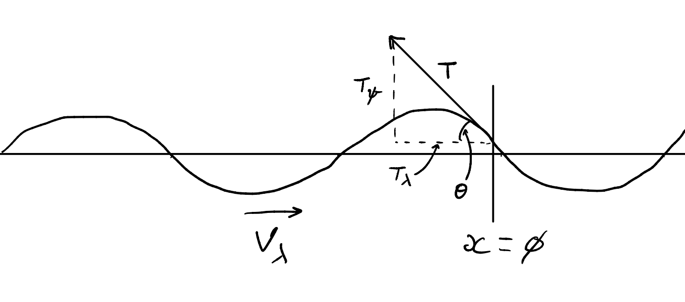
Fig. 16 Wave travelling from left to right with velocity \(v_\lambda\) in a wire under tension, \(T\). Note the direction of \(T\) at point \(x=0\) which I have shown as the large arrow. I have decomposed this force into its vertical, \(T_\psi\) and horizontal, \(T_\lambda\) components.

Firstly, all waves aside, you will recall from your pre-university days that a force, \(F\), acting over a distance, \(\Delta L\), expends an energy \(\Delta E=F\Delta L\). You will also recall that power is energy per unit time, or

(89)\[\begin{split}\begin{align} P &= \frac{\Delta E}{\Delta t} \nonumber\\ &=\frac{F\Delta L}{\Delta t}\nonumber\\ &=Fv\label{fv} \end{align}\end{split}\]

where \(\Delta t\) is change in time and \(v=\Delta L/\Delta t\) is velocity.

Now, let’s return to the wire in question. Remember that, while the wave travels horizontally along the wire at a velocity, \(v_\lambda=\omega/k\), the wire itself only moves vertically. You can think of this in terms of just a small section of the wire at \(x=0\): as the wave passes from left-to-right, the section only moves up and down. Since it is located at \(x=0\) the displacement of this section of the wire at time \(t\) is simply:

(90)\[\begin{equation} \label{displacement} \psi(t) = \psi_0\sin(-\omega t). \end{equation}\]

It is important to appreciate that the work that the wave does is in making that section of the wire move up-and-down. To help understand this point, it may be helpful to think in terms of how you would actually get energy out of such a system. You could, for example, place a small mass on the wire at \(x=0\). As the wave travelled past, it would lift the mass against the force of gravity and therefore do work.

As a consequence, the velocity that goes into Eq. (89) is not the velocity of the wave, but the vertical velocity of the wire as the wave passes, which we’ll denote \(v_\psi\). Just as in a mass-on-spring SHO, the vertical velocity is given by differentiating the displacement with respect to time

(91)\[\begin{split}\begin{align} v_\psi &= \frac{d\psi(t)}{dt}\\\nonumber &= -\omega\psi_0\cos(-\omega t)\label{vv}. \end{align}\end{split}\]

Now we’ll turn our attention to the force part of Eq. (91). Ignoring gravity,[1] the only force within this system is the tension in the wire, \(T\). Recall, however, that when we calculate work done, we only consider the component of the force that is in the same direction as the displacement \(\Delta L\).[2] Since we’ve already established that the work done is in moving the wire up-and-down, we therefore need to derive the vertical component of the tension.

Considering Fig. 16 for a moment, we see that the vertical component of the tension, \(T_\psi\), is equal to \(-T\sin(\theta(x=0,t))\), where \(\theta(x=0,t)\) is angle between the wire at \((x=0,t)\) and the horizontal. The negative sign is in there because the \(x\) component of \(T\) always points from right-to-left (i.e., along the negative \(x\) direction). Calculating \(\sin(\theta(x,t))\) from the wave equation is quite hard, but can be made much easier if \(\theta(x,t)\) is always small, in which case \(\sin(\theta(x,t))\approx\tan(\theta(x,t))\). What this means physically is that the wavelength of the wave is much longer than the amplitude of the wave; if that’s not the case then the following maths doesn’t work.

The reason why adopting \(\sin(\theta(x,t))\approx\tan(\theta(x,t))\) makes things easier for us is that \(\tan(\theta(x,t))\) is simply the gradient of the wire evaluated at position \(x\). And the gradient is obtained by differentiating the displacement of the wire with respect to \(x\), i.e.,

(92)\[\begin{align} \tan(\theta(x,t)) &= \frac{dy}{dx}\nonumber\\ &=\frac{d\psi}{dx}\nonumber\\ &=k\psi_0\cos(kx-\omega t). \end{align}\]

Therefore the vertical component of the tension at \(x=0\) is

(93)\[\begin{align} T_\psi &=-T\sin(\theta(x=0,t))\nonumber \\ &\approx-T\tan(\theta(x=0,t)\nonumber \\ &\approx-Tk\psi_0\cos(-\omega t). \end{align}\]

Now that we have expressions for \(F\) (which is equal to \(T_\psi\)) and \(v_\psi\), we can combine them according to Eq. (89) to get

(94)\[\begin{align} P&=F_Vv_\psi\nonumber \\ &=T_\psi v_\psi\nonumber \\ &\approx -\omega\psi_0\cos(-\omega t)\cdot -Tk\psi_0\cos(-\omega t)\nonumber \\ &\approx Tk\omega\psi_0^2\cos^2(-\omega t) \nonumber \\ &\approx \mu v_\lambda\omega^2A^2\cos^2(-\omega t), \end{align}\]

where the last step has used \(v_\lambda=\omega/k\) and \(T=\mu v_\lambda^2\), where \(v_\lambda\) is the velocity of the wave and \(\mu\) is the mass per unit length of the wire.[3]

You’ll notice that the above expression for power is time-dependent, in other words it changes with time via the \(\cos^2(-\omega t)\). As such, the instantaneous power transmission of a wave changes throughout its cycle. Normally, however, we don’t measure the instantaneous power transmission of a wave, but rather the power averaged over multiple cycles. This is certainly true of light waves and sound waves, and indeed most mechanical waves. To calculate the average power transmission of the wave, \(\langle P\rangle\), we need to calculate the average of \(\cos^2(\omega t)\) over an integer number of cycles (i.e., from \(\omega t = 0\) to \(\omega t = 2n\pi\), where \(n\) is an integer). Doing this requires the use of compound angle formulae, which I’m not going to go into here, but it ultimately boils down to

(95)\[\begin{align} \langle f(\epsilon)\rangle &=\frac{1}{b-a}\int_a^bf(\epsilon)d\epsilon\nonumber \\ &=\frac{1}{2n\pi-0}\int_0^{2n\pi}\cos^2(\epsilon) d\epsilon\nonumber\\ &=\frac12, \end{align}\]

where I’ve just used \(\epsilon\) to mean “any variable”, as I didn’t want to use a parameter that I had used before in this lecture’s notes.[4]

Since the average of \(\cos^2(-\omega t)\) over multiple cycles is \(1/2\), then the average power output of a mechanical wave is

(96)\[\begin{align} \langle P\rangle &\approx\langle \cos^2(-\omega t)\rangle Tk\omega\psi_0^2\nonumber\\ &\approx\frac{1}{2}Tk\omega\psi_0^2\nonumber\\ &\approx\frac{1}{2}\mu v_\lambda\omega^2A^2. \end{align}\]

Summary

In this lecture we have seen how we can derive the average power output of a mechanical wave by considering the forces acting upon a section of wire and the rate of change of displacement of the wire (\(v_\psi\)). While deriving the power output of different types of waves requires different expressions for force and displacement, they all involve similar considerations. For example, electromagnetic waves induce an electrostatic force, while sound waves induce a force due to pressure. What does carry over into all types of waves is that the power output is always proportional to the square of the amplitude of the wave - a result of multiplying the spatial and temporal derivatives of the wave equation.

This lecture marks a transition point in the lecture series. Since you should, by now, have learned about Euler’s formula in PHY120, then from next lecture onwards we’ll see how we can use complex numbers to describe waves. As we shall see, this will allow us to tackle some oscillating systems that would otherwise prove very difficult with trig. functions alone.

---

[1]

The wave would travel along the wire irrespective of whether it were in a gravitational field or not.

[2]

More specifically, work done is the scalar product of force and displacement.

[3]

\(T=\mu v_\lambda^2\) just comes from the expression for the velocity of a wave in a wire under tension. I haven’t derived it.

[4]

You may wish to prove the above yourself.