2 - Simple Harmonic Motion and the Small Angle Approximation

What causes Simple Harmonic Motion?

In the previous lecture, we looked at our first examples of oscillators and focussed on the specific case of a harmonic oscillator. These are oscillators whose displacement is described as sinusoidal. While we considered a few examples of hormonic oscillators such as masses on springs and pendula – we didn’t look at why these and other systems are harmonic oscillators. Clearly, not all systems undergo oscillatory motion when ‘nudged’; a ball, when thrown, does not reach a maximum distance then return to the thrower. So what conditions are needed for a system to undergo harmonic oscillations?

It turns out that a system undergoes harmonic motion if there exists a force pulling it back toward an equilibrium position, and that the magnitude of that force is proportional to the extent by which the system is displaced from its equilibrium position. I’ve intentionally tried to make that last statement as general as I can, but sometimes being general isn’t very helpful when you’re trying to teach a concept. So, let’s be more specific and think of our go-to oscillator – that which consists of a mass tied to a spring.

Before I start the mass-on-spring oscillating, it rests – unmoving – at its equilibrium position. At this position, the force due to gravity is balanced by the tension in the spring which, via Hooke’s Law, is proportional to the extension of the spring. If I pull the mass downwards, I can feel the force from the spring increasing in strength as I pull it farther away from its equilibrium position. And crucially, this force is in the opposite direction – upwards – to the direction I am pulling the mass and is – because of Hooke’s Law – proportional to its distance from equilibrium. The same happens if I push the mass upwards – again, the force from the spring is in the opposite direction – now downwards – to the direction I am pushing the mass. It is this ‘proportional-but-opposite direction’ force – also known as a restoring force – that causes the mass-on-spring system to oscillate harmonically. But of course, this is not just restricted to masses on springs – all harmonic oscillators have, if you look deeply enough, a proportional restorative force at their hearts.

Because we’re physicists we can use maths to describe the ‘proportional-but-opposite direction’ forces that cause a system to oscillate harmonically. In the case of a mass on a spring, the restoring force is \(F_k=-kx\) where \(k\) is the spring constant and \(x\) is the displacement from equilibrium. The minus sign is in there because the force, \(F_k\), is in the opposite direction to the displacement, \(x\). If we next add Newton’s Second Law of Motion – the \(F=ma\) one – to the mix, we get:

(13)\[\begin{equation} \label{ma} ma = -kx \end{equation}\]

where \(a\) is the acceleration of the mass, \(m\). Remembering that acceleration is the time derivative of velocity, \(v\), and that velocity is the time derivative of distance (or, more specifically, displacement), Eq. (13) becomes:

\[\begin{equation} ma = m\frac{dv}{dt}=m\frac{d^2x}{dt^2} = -kx \end{equation}\]

or, equivalently:

(14)\[\begin{equation} \label{fracd2} \frac{d^2x}{dt^2} + \frac{k}{m}x = 0. \end{equation}\]

What I like about the above Eq. (14) is that, while we derived it using the mass-on-spring system, its constituent terms – \(k\) and \(x\) – look very generic, so it’s easy to see how this same equation can be applied to any system that has a ‘proportional-but-opposite direction’ force.

Equation (14) is known as a second-order ordinary differential equation. Later, you’ll learn how to solve differential equations to show that \(x=A\,{\rm sin}(\omega t)\) is a general solution to Eq. (14). In doing so, you’ll demonstrate that a system that obeys Eq. (14) undergoes sinusoidal – or, harmonic – oscillations. For now, however, we’ll take the easy route and show it by substituting \(x=A\,{\rm sin}(\omega t)\) into Eq. (14).

(15)\[\begin{equation} -A\omega^2\,{\rm sin}(\omega t) + \frac{k}{m} A\,{\rm sin}(\omega t)= 0. \end{equation}\]

Cancelling the \(A\,{\rm sin}(\omega t)\)’s, and adding \(\omega^2\) to both sides gives:

(16)\[\begin{equation} \frac{k}{m} = \omega^2 \end{equation}\]

or

(17)\[\begin{equation} \omega = \sqrt{\frac{k}{m}}, \end{equation}\]

meaning that \(x=A{\rm sin}(\omega t)\) is a solution to Eq. (14) when \(\omega=\sqrt{k/m}\).

The Pendulum

Perhaps the most famous of all harmonic oscillators is the pendulum - a mass, \(m\), at the end of a piece of string or rod that moves to and fro. Presumably this most prototypical harmonic oscillator must be dictated by a ‘proportional-but-opposite direction’ force? Well, yes – and no. To see why it’s not a straightforward ‘yes’, we need to look closely at the forces acting on a pendulum (see Fig. 5).

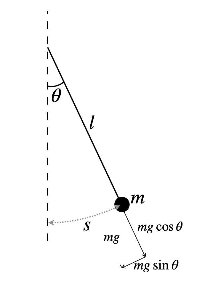
Fig. 5 A pendulum consisting of a mass, \(m\), at the end of a light (i.e., massless) piece of string or rod of length \(l\). In this figure, the pendulum is shown displaced from its equilibrium position by an angle, \(\theta\), corresponding to an arc of length \(s\).

It’s clear that as the pendulum moves away from its equilibrium position, the force of gravity, \(F_{g}=mg\), tries to pull the pendulum back to its equilibrium position. With the pendulum now at an angle from its equilibrium position, this force can be decomposed into two components, a component pointing in the direction parallel to the rod, \(mg\,\rm{cos(\theta)}\), and another pointing in the direction perpendicular to the rod toward the equilibrium position, \(-mg\,\rm{sin(\theta)}\). The negative sign in there is because the horizontal force is in the opposite direction to the displacement from equilibrium.

So, \(-mg\,\rm{sin(\theta)}\), is the restorative force, but what about the \(F=ma\) part or, more specifically, the acceleration? As it moves, the pendulum traces-out a section of a circle. As we saw in the last lecture, this section of circle is given by \(s=\theta l\), where \(l\) is the length of the pendulum, and \(\theta\) is the angle – measured in radians – that the pendulum subtends from the vertical. This means that the acceleration is given by:

(18)\[\begin{equation} a = \frac{d^2 s}{dt^2} = l\frac{d^2\theta}{dt^2}. \end{equation}\]

Equating the restorative force due to gravity with \(F=ma\) gives, therefore,

(19)\[\begin{equation} ml\frac{d^2\theta}{dt^2} = -mg\,{\rm sin}(\theta). \end{equation}\]

Cancelling the \(m\)’s and adding \(g\,{\rm sin}(\theta)\) to both sides, and dividing by \(l\) gives:

(20)\[\begin{equation} \label{pendulumexact} \frac{d^2\theta}{dt^2} + \frac{g}{l}\,{\rm sin}(\theta) = 0 \end{equation}\]

which looks almost, but not quite, like Eq. (14). The problem is the \({\rm sin}(\theta)\) which means that the restorative force is not proportional to the distance from equilibrium. What’s going on? If it doesn’t obey the ‘proportional-but-opposite direction’ rule, then why is a pendulum used throughout physics (and clockmaking) as an example of a harmonic oscillator? For that, we need to consider some really small angles. First, however, an aside…

A secret about your degree

I’m going to let you into a secret about your degree. The secret is that the most important thing we teach you in a Physics degree is not Physics. Instead, the most important thing you get from a Physics degree is a set of tools that you can use to ‘do’ Physics; the Physics ‘knowledge’ is a by-product that makes using the tools interesting. I’m not, of course, referring to a literal set of tools but a set of techniques that you’ll have at your disposal to solve problems. Throughout your degree, you’ll learn how to program computers to solve just about any problem you can think of, and how to use maths to not just model physical systems, but anything that can be broken down into simpler interactions such as financial markets or disease transmission.

This ‘tool acquisition’ is particularly prominent during the first two years of your degree, and perhaps even more-so in the Waves and Oscillations part of PHY11006. You may think I introduced the pendulum in the previous section because it’s a classic example of a harmonic oscillator. In fact, I’m going to use it demonstrate the importance of a new tool I’m going to teach you in the next section. Hopefully, you’ll learn to use it proficiently (and eventually without even thinking) during your degree and, if you wish, for a long time afterwards. Indeed, I still use it almost daily in my research, but then, I’m an astronomer!

Aside: Maclauren and Taylor series

Note: You won’t be examined on the Maclauren or Taylor Series in your Waves and Oscillations exam question.

Throughout your degree, you’ll encounter many physics problems which, in their exact forms, are extremely difficult or even impossible to solve. These are known as ‘intractable’ problems. The Universe is full of intractable problems – unfortunately, the Universe plays by its own rules and doesn’t give a jott about whether it is easy to solve! Equation (20) is an example of an intractable problem – it is really hard to solve this differential equation analytically to get an exact answer; indeed, it might even be impossible (I’ve never tried).

Rather than give up, however, physicists have figured out a number of ways of approximating intractable problems so that they are easy or, at least, possible to solve. Often this means that they concede that they can solve a problem provided that its parameters satisfy some reasonable criteria. As we’ll see, the pendulum is an example of one such system.

To make Eq. (20) solvable, we are going to use a Maclauren series to obtain an approximation of the \(\sin(\theta)\), since that’s the part that makes the problem intractable. A Maclauren series is a specific case of a broader class known as Taylor series. The underlying premise of both Maclauren and Taylor series is that any well-behaved[1] function can be re-written as a polynomial containing an infinite number of terms, i.e.,

(21)\[\begin{equation} \label{polynomial} f(x) = a_0 + a_1x + a_2x^2 + a_3x^3\dots a_nx^n. \end{equation}\]

A rigorous proof of this premise is beyond the scope of this module, but hopefully you can already see why it at least makes some kind of sense. Imagine a well-behaved function that has an offset, some straightish bits, some curved bits, and some inversions (where the line changes direction). Well, provided the constants \(a_n\) are appropriate, the \(a_0\) part in Eq. (21) will deal with the offset, the \(a_1x\) part will deal with the straight bits, while the \(a_2x^2\) and \(a_3x^3\) will take care of the curves and inversions. The more squiggly your function, the more important the later terms are, and you can keep adding terms until you get as good a representation as you like. For many functions you won’t get an exact representation of \(f(x)\) unless you have an infinite number of terms, but often in physics we don’t need an exact representation.

With the Maclauren and Taylor series, the hard work is trying to work out what are appropriate values for the constants. In the case of \(a_0\) in Eq. (21) this is fairly straightforward, you simply set \(x=0\) and all the higher order terms (i.e., \(a_1x\) onwards) disappear, meaning,

(22)\[\begin{equation} f(0) = a_0, \end{equation}\]

with \(f(0)\) simply meaning the value of \(f(x)\) when \(x=0\) (we usually say ‘evaluated at zero’). For the higher terms, we can use a nice feature of differentiation. If we differentiate both sides or Eq. (21) with respect to \(x\), we get:

(23)\[\begin{equation} \frac{df(x)}{dx} = f^\prime(x) = a_1 + 2a_2x + 3a_3x^2 + \dots+ na_nx^{n-1}, \end{equation}\]

where I’ve used the \(f^\prime(x)\) notation to mean the first derivative of \(f(x)\) with respect to \(x\). Now if we set \(x=0\), the higher order terms disappear and we get:

(24)\[\begin{equation} f^\prime(0) = a_1, \end{equation}\]

meaning that the value for the constant \(a_1\) is obtained by differentiating \(f(x)\) with respect to \(x\), then evaluating that derivative at \(x=0\). For \(a_2\) we can do the same, remembering, however, about the constants introduced due to differentiation:

(25)\[\begin{equation} f''(x) = 2a_2 + 6a_3x + \dots+ n(n-1)a_nx^{n-2}, \end{equation}\]

meaning when we set \(x=0\), then

(26)\[\begin{equation} \frac{f''(0)}{2} = a_2. \end{equation}\]

We can keep differentiating-then-setting-zero ad-infinitum to get as many constants as we like:

(27)\[\begin{equation} f(x) = f(0) + f'(0)x + \frac{f''(0)}{2}x^2 + \frac{f'''(0)}{2\times3}x^3\dots . \end{equation}\]

You should be able to see that the denominator for the fourth term will be \(2\times3\times4\) and subsequent ones will increase as factorials (i.e., as \(n!\)). We can therefore concisely write this series as:

(28)\[\begin{equation} f(x) = \sum_{n=0}^{\infty} \frac{f^n(0)x^n}{n!} . \end{equation}\]

where \(f^n(0)\) means the nth-derivative of \(f(x)\) evaluated at zero.

Of course, you’re not going to want to differentiate \(f(x)\) an infinite number of times. If you’re happy to differentiate it \(N\) times instead, then what you get is an approximation of \(f(x)\), i.e.,

(29)\[\begin{equation} \label{maclauren} f(x) \approx \sum_{n=0}^{N} \frac{f^n(0)x^n}{n!} . \end{equation}\]

Typically, the more terms you have, the further away from zero you can take \(x\) without getting too far away from the true value of \(f(x)\).

Equation (29) is the Maclauren series – it deals with approximating a function close to zero. The Taylor series, by contrast, is more general: it deals with approximating a function close to any value. The Taylor series is given by:

(30)\[\begin{equation} \label{taylor} f(x) \approx \sum_{n=0}^{N} \frac{f^n(b)(x-b)^n}{n!} . \end{equation}\]

Here, \(x\) needs to be close to \(b\), rather than 0, in order for the approximation to hold.

Back to the pendulum

With the Taylor, and more specifically, Maclauren series in our tool-belt, we can now return to the problem of the simple pendulum. As long as we don’t displace the pendulum by too much – in other words, as long as \(\theta\) stays small and doesn’t depart too much from zero – then we can use a Maclauren series to approximate the \(\sin(\theta)\) in Eq. (20). Recalling that the first derivative of \(\sin(\theta)\) is \(\cos(\theta)\), and the second derivate is \(-\sin(\theta)\), the process in full looks like:

(31)\[\begin{align} \sin(\theta)&=\sin(0) + \cos(0)\theta - \frac{\sin(0)}{2}\theta^2 - \frac{\cos(0)}{2\times3}\theta^3+\dots\nonumber\\ &=0 + \theta - 0 - \frac{\theta^3}{6}+\dots\nonumber\\ &=\theta - \frac{\theta^3}{6}+\dots . \end{align}\]

If we then state that \(\theta=0.17\)~rad, or about 10 degrees, then this becomes

(32)\[\begin{equation} 0.17 - 8.188333\times10^{-4} + \dots . \end{equation}\]

There are two things to notice here, the first is that \(0.17 - 8.188333\times10^{-4}=0.169181\), whereas \(\sin(0.17)=0.169182\), meaning that with just two non-zero terms, we’re already within \(0.0008\%\) of the true value of \(\sin(0.17)\)![2] The second thing to notice is that \(8.2\times10^{-4}\) is about two hundred times smaller than 0.17, so if we had only taken the first non-zero term, we’d still easily be within \(1\%\) of the true value of \(\sin(0.17)\). As such, provided we keep \(\theta\) below about 10 degrees, we can adopt the approximation \(\sin(\theta)\approx\theta\), and still be confident that our equations are valid to one part in at least 100.

Using the \(\sin(\theta)\approx\theta\) approximation, Eq. (20) becomes

(33)\[\begin{equation} \label{pendulumapprox} \frac{d^2\theta}{dt^2} + \frac{g}{l}\theta = 0 \end{equation}\]

which does indeed look like Eq. (14). I’ll leave it to you to show – by substitution – that \(\theta(t)=\theta_0\sin(\omega t)\) is a solution to Eq. (33), where \(\theta_0\) is the maximum angular displacement. However, by simply comparing it to Eq. (14), you should be able to see that \(\theta(t)=\theta_0\sin(\omega t)\) is a solution when

(34)\[\begin{equation} \omega = \sqrt\frac{g}{l}. \end{equation}\]

---

[1]

A well-behaved function is typically defined as one that is single-valued (i.e., there’s only one value of y for every value of x), continuous (i.e., doesn’t contain breaks), and varies smoothly (i.e., doesn’t contain ‘steps’)

[2]

I’ve written \(8.188333\times10^{-4}\) to an inappropriately large number of significant figures to show how far I needed to go to get to the first different decimal place.